pacman::p_load(
      here,      # file locator
      tidyverse, # data management and ggplot2 graphics
      skimr,     # get overview of data
      janitor,   # produce and adorn tabulations and cross-tabulations
      tsibble,
      fable,
      feasts
)

covid_data <- readRDS(here("data", "clean", "final_covid_data.rds"))ACF and PACF plots
Load packages and data:
The ACF and PACF plots should be considered together.
For the AR process in the ARIMA, we expect that the ACF plot will gradually decrease and simultaneously the PACF should have a sharp drop after p significant lags.
To define a MA process in the ARIMA, we expect the opposite from the ACF and PACF plots, meaning that: the ACF should show a sharp drop after a certain q number of lags while PACF should show a geometric or gradual decreasing trend.
On the other hand, if both ACF and PACF plots demonstrate a gradual decreasing pattern, then the ARMA process should be considered for modeling.
Asturias
data_asturias <- covid_data %>%
      filter(provincia == "Asturias") %>%
      select(provincia, fecha, num_casos, num_hosp, tmed,mob_grocery_pharmacy, mob_parks,
             mob_residential, mob_retail_recreation, mob_transit_stations, mob_workplaces, mob_flujo) %>%
      # Drop NAs dates except for mob_flujo since the data finish in 2021 while other sources are ut to 31/03/2022
      drop_na(-mob_flujo) %>%
      as_tsibble(key = provincia, index = fecha)
data_asturias
# A tsibble: 774 x 12 [1D]
# Key: provincia [1]
provincia fecha num_casos num_hosp tmed mob_grocery_pharmacy mob_parks
<chr> <date> <dbl> <dbl> <dbl> <dbl> <dbl>
1 Asturias 2020-02-15 0 0 12.2 -1 20
2 Asturias 2020-02-16 0 0 16.2 1 11
3 Asturias 2020-02-17 0 2 9.8 0 -13
4 Asturias 2020-02-18 0 0 8.8 1 11
5 Asturias 2020-02-19 0 0 8.6 1 29
6 Asturias 2020-02-20 0 0 9.9 0 32
7 Asturias 2020-02-21 0 0 11.2 -1 18
8 Asturias 2020-02-22 0 0 10.5 1 29
9 Asturias 2020-02-23 1 0 9.2 6 23
10 Asturias 2020-02-24 0 0 8.6 5 48
# … with 764 more rows, and 5 more variables: mob_residential <dbl>,
# mob_retail_recreation <dbl>, mob_transit_stations <dbl>,
# mob_workplaces <dbl>, mob_flujo <dbl># ACF
data_asturias %>%
ACF(num_casos, lag_max = 30) %>%
autoplot() +
labs(title=" Asturias - ACF Nº Cases")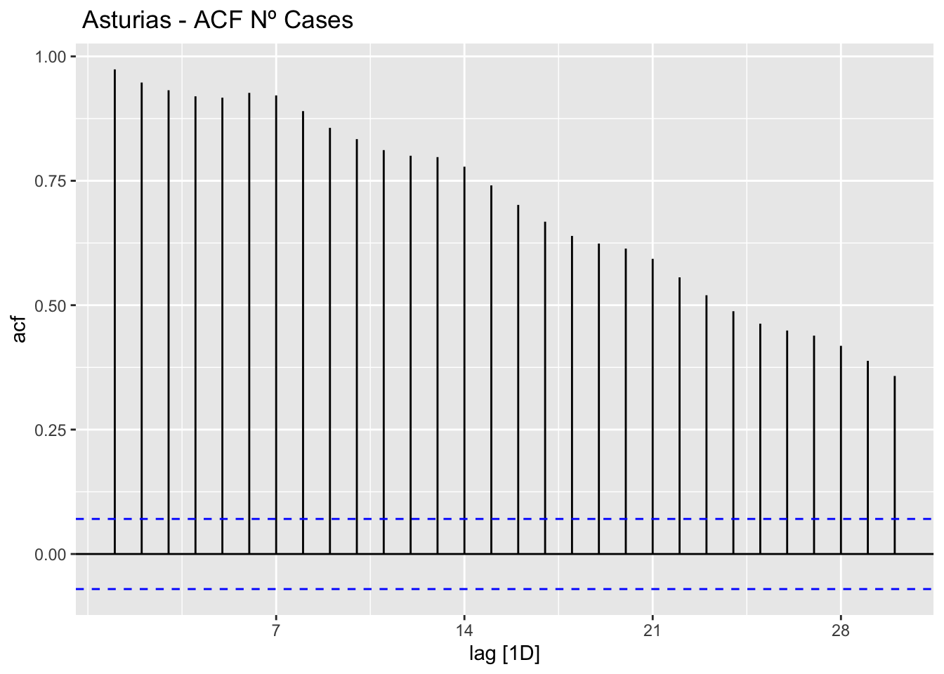
# PACF
data_asturias %>%
      PACF(num_casos, lag_max = 30) %>%
      autoplot() +
      labs(title=" Asturias - PACF Nº Cases")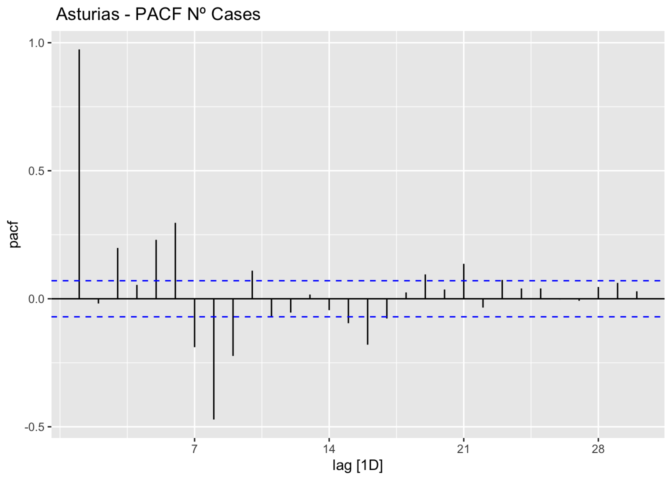
Barcelona
data_barcelona <- covid_data %>%
      filter(provincia == "Barcelona") %>%
      select(provincia, fecha,num_casos, num_hosp, tmed, mob_grocery_pharmacy, mob_parks,
             mob_residential, mob_retail_recreation, mob_transit_stations, mob_workplaces, mob_flujo) %>%
      # Drop NAs dates except for mob_flujo since the data finish in 2021 while other sources are ut to 31/03/2022
      drop_na(-mob_flujo) %>%
      as_tsibble(key = provincia, index = fecha)
data_barcelona
# A tsibble: 774 x 12 [1D]
# Key: provincia [1]
provincia fecha num_casos num_hosp tmed mob_grocery_pharmacy mob_parks
<chr> <date> <dbl> <dbl> <dbl> <dbl> <dbl>
1 Barcelona 2020-02-15 12 4 12.8 -3 14
2 Barcelona 2020-02-16 2 4 14.5 -8 2
3 Barcelona 2020-02-17 1 5 14.6 1 11
4 Barcelona 2020-02-18 5 7 11.5 1 8
5 Barcelona 2020-02-19 1 8 11.8 1 6
6 Barcelona 2020-02-20 11 10 10.4 1 9
7 Barcelona 2020-02-21 15 8 11.9 -1 11
8 Barcelona 2020-02-22 8 10 12 -1 25
9 Barcelona 2020-02-23 7 8 12.9 0 26
10 Barcelona 2020-02-24 8 4 13.6 1 21
# … with 764 more rows, and 5 more variables: mob_residential <dbl>,
# mob_retail_recreation <dbl>, mob_transit_stations <dbl>,
# mob_workplaces <dbl>, mob_flujo <dbl># ACF
data_barcelona %>%
ACF(num_casos, lag_max = 30) %>%
autoplot() +
labs(title=" Barcelona - ACF Nº Cases")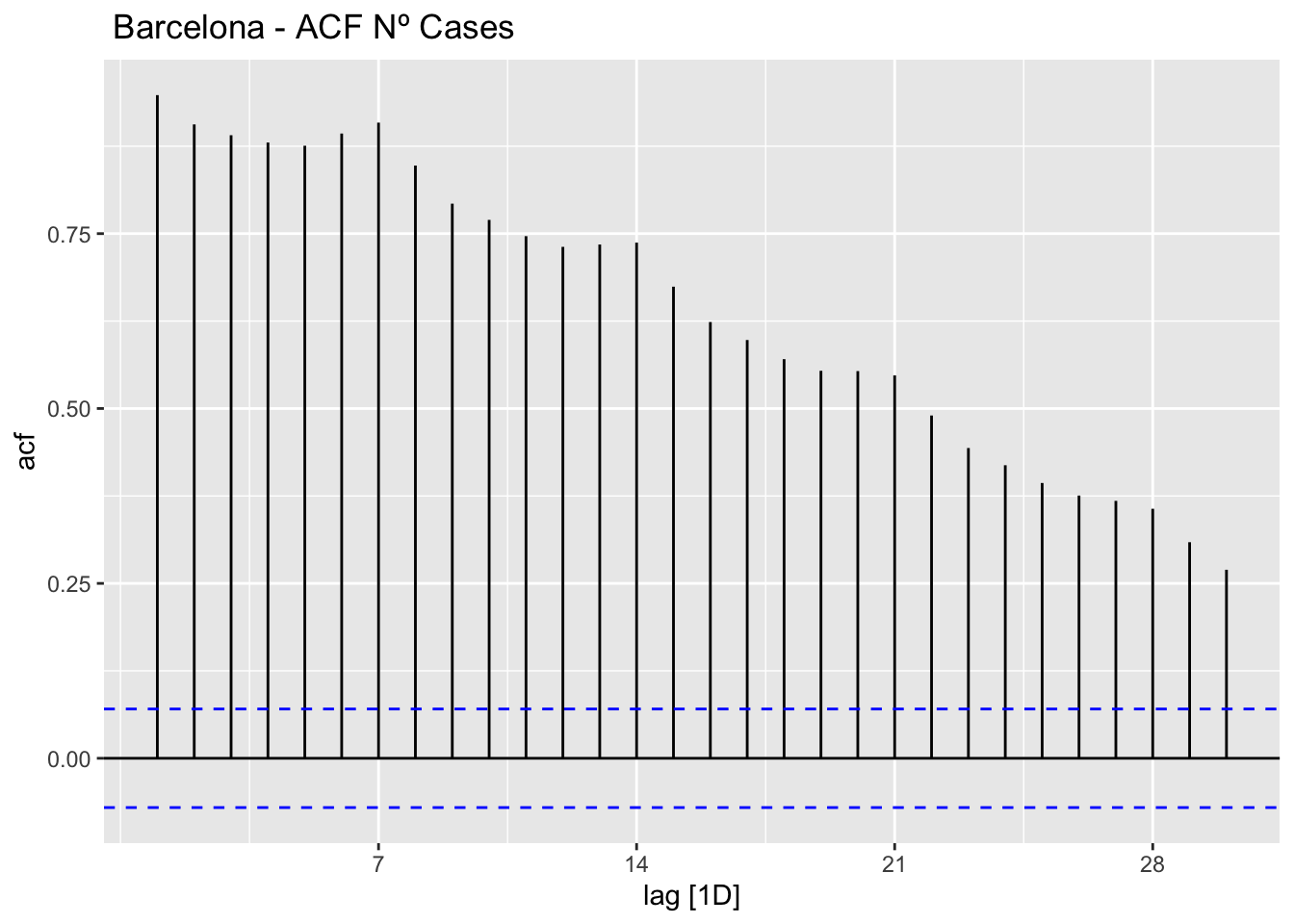
data_barcelona %>%
      PACF(num_casos, lag_max = 30) %>%
      autoplot() +
      labs(title=" Barcelona - PACF Nº Cases")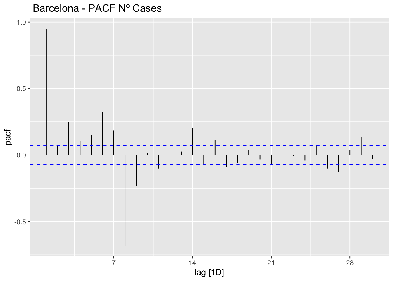
Madrid
data_madrid <- covid_data %>%
      filter(provincia == "Madrid") %>%
      select(provincia, fecha, num_casos, num_hosp, tmed, mob_grocery_pharmacy, mob_parks,
             mob_residential, mob_retail_recreation, mob_transit_stations, mob_workplaces, mob_flujo) %>%
      # Drop NAs dates except for mob_flujo since the data finish in 2021 while other sources are ut to 31/03/2022
      drop_na(-mob_flujo) %>%
      as_tsibble(key = provincia, index = fecha)
data_madrid
# A tsibble: 774 x 12 [1D]
# Key: provincia [1]
provincia fecha num_casos num_hosp tmed mob_grocery_pharmacy mob_parks
<chr> <date> <dbl> <dbl> <dbl> <dbl> <dbl>
1 Madrid 2020-02-15 13 4 8.6 -2 31
2 Madrid 2020-02-16 13 2 9.6 4 34
3 Madrid 2020-02-17 19 9 9.1 3 10
4 Madrid 2020-02-18 14 13 8.5 1 11
5 Madrid 2020-02-19 12 14 8.6 1 18
6 Madrid 2020-02-20 25 15 8 1 18
7 Madrid 2020-02-21 26 18 10.4 1 22
8 Madrid 2020-02-22 29 8 10.8 -1 53
9 Madrid 2020-02-23 44 8 11.6 6 56
10 Madrid 2020-02-24 56 18 10.8 6 35
# … with 764 more rows, and 5 more variables: mob_residential <dbl>,
# mob_retail_recreation <dbl>, mob_transit_stations <dbl>,
# mob_workplaces <dbl>, mob_flujo <dbl># ACF
data_madrid %>%
ACF(num_casos, lag_max = 30) %>%
autoplot() +
labs(title=" Madrid - ACF Nº Cases")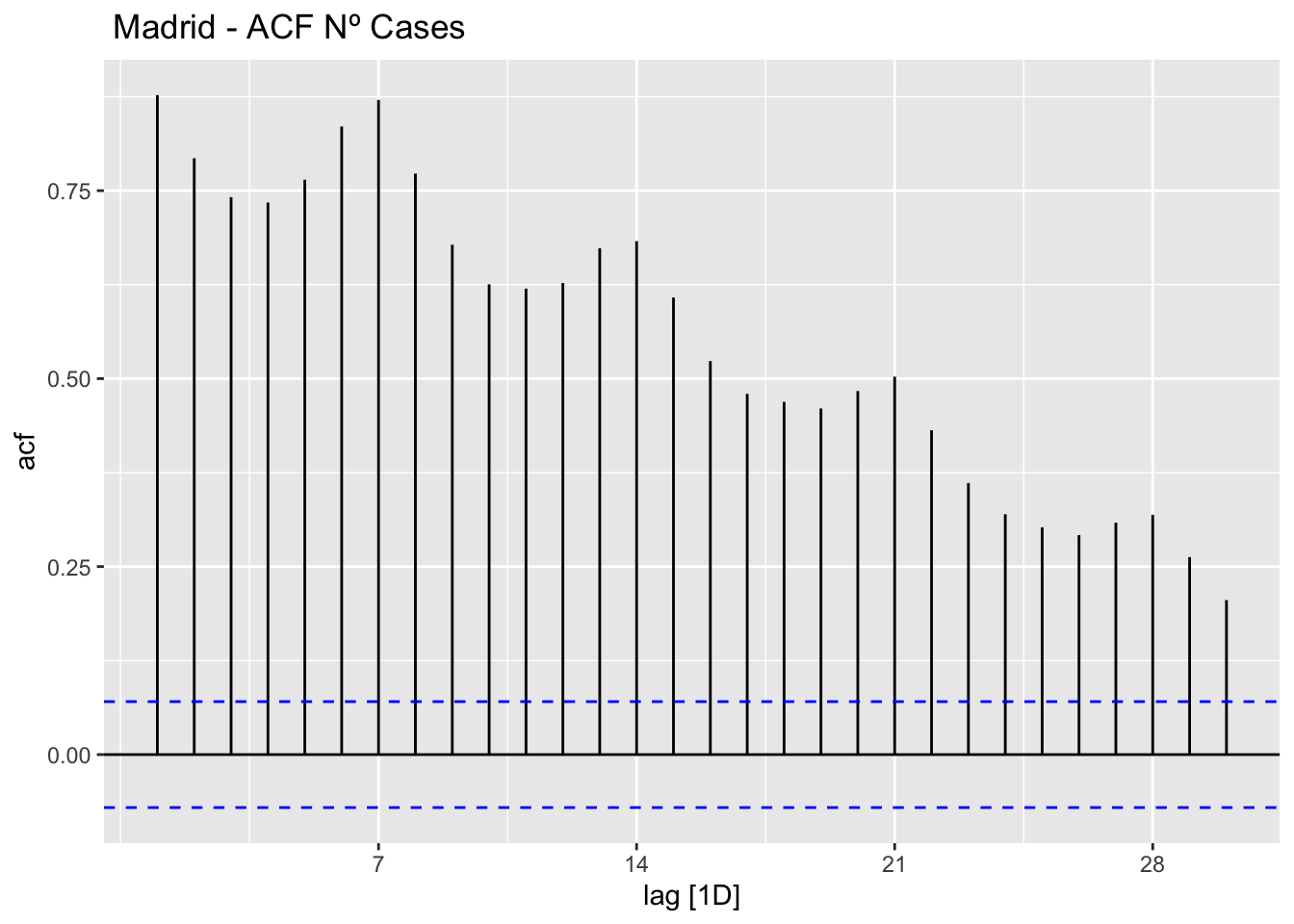
# PACF
data_madrid %>%
      PACF(num_casos, lag_max = 30) %>%
      autoplot() +
      labs(title=" Madrid - PACF Nº Cases")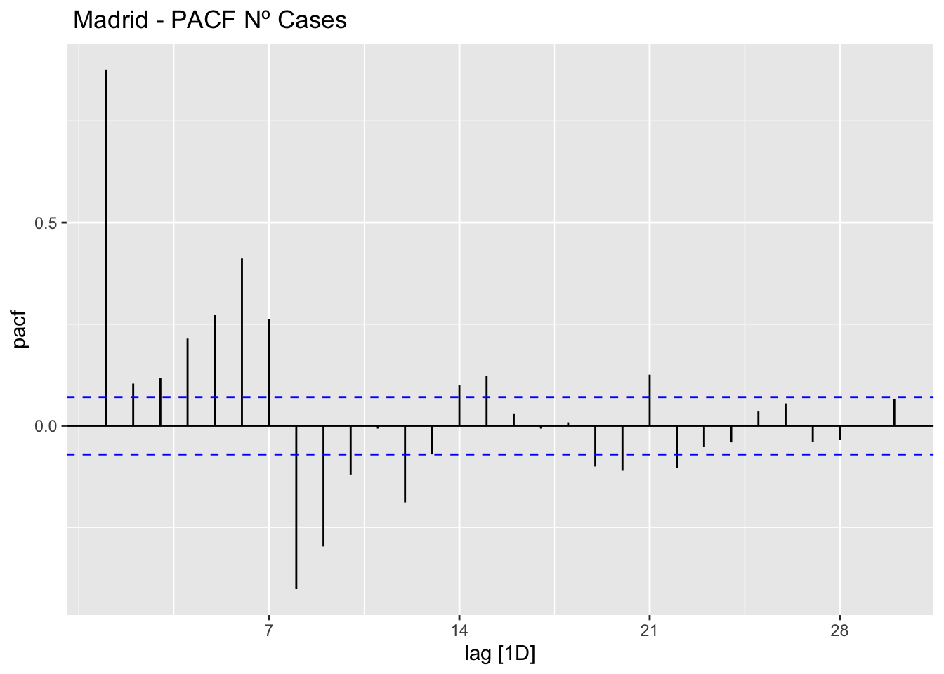
Málaga
data_malaga <- covid_data %>%
      filter(provincia == "Málaga") %>%
      select(provincia, fecha, num_casos, num_hosp, tmed, mob_grocery_pharmacy, mob_parks,
             mob_residential, mob_retail_recreation, mob_transit_stations, mob_workplaces, mob_flujo) %>%
      # Drop NAs dates except for mob_flujo since the data finish in 2021 while other sources are ut to 31/03/2022
      drop_na(-mob_flujo) %>%
      as_tsibble(key = provincia, index = fecha)
data_malaga
# A tsibble: 774 x 12 [1D]
# Key: provincia [1]
provincia fecha num_casos num_hosp tmed mob_grocery_pharmacy mob_parks
<chr> <date> <dbl> <dbl> <dbl> <dbl> <dbl>
1 Málaga 2020-02-15 1 0 13.5 0 29
2 Málaga 2020-02-16 0 0 14 4 16
3 Málaga 2020-02-17 0 0 17.1 1 14
4 Málaga 2020-02-18 0 0 15.4 0 -1
5 Málaga 2020-02-19 0 2 15.9 0 -1
6 Málaga 2020-02-20 1 0 14.9 1 13
7 Málaga 2020-02-21 3 2 13.6 -1 3
8 Málaga 2020-02-22 2 1 14.2 -1 25
9 Málaga 2020-02-23 2 0 13.2 10 15
10 Málaga 2020-02-24 2 1 14 0 22
# … with 764 more rows, and 5 more variables: mob_residential <dbl>,
# mob_retail_recreation <dbl>, mob_transit_stations <dbl>,
# mob_workplaces <dbl>, mob_flujo <dbl># ACF
data_malaga %>%
ACF(num_casos, lag_max = 30) %>%
autoplot() +
labs(title=" Malaga - ACF Nº Cases")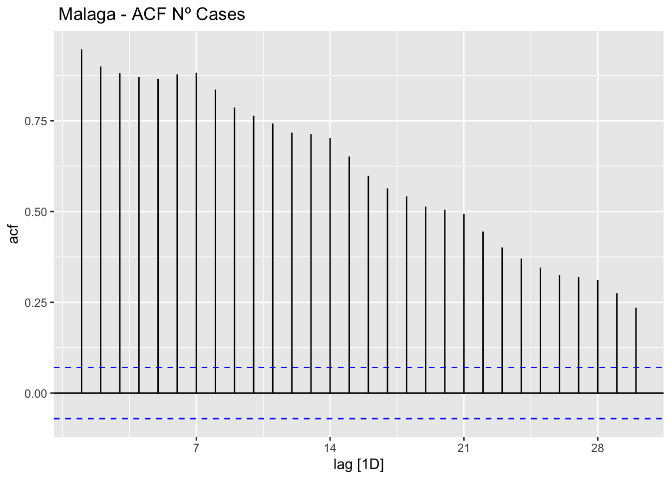
# PACF
data_malaga %>%
      PACF(num_casos, lag_max = 30) %>%
      autoplot() +
      labs(title=" Malaga - PACF Nº Cases")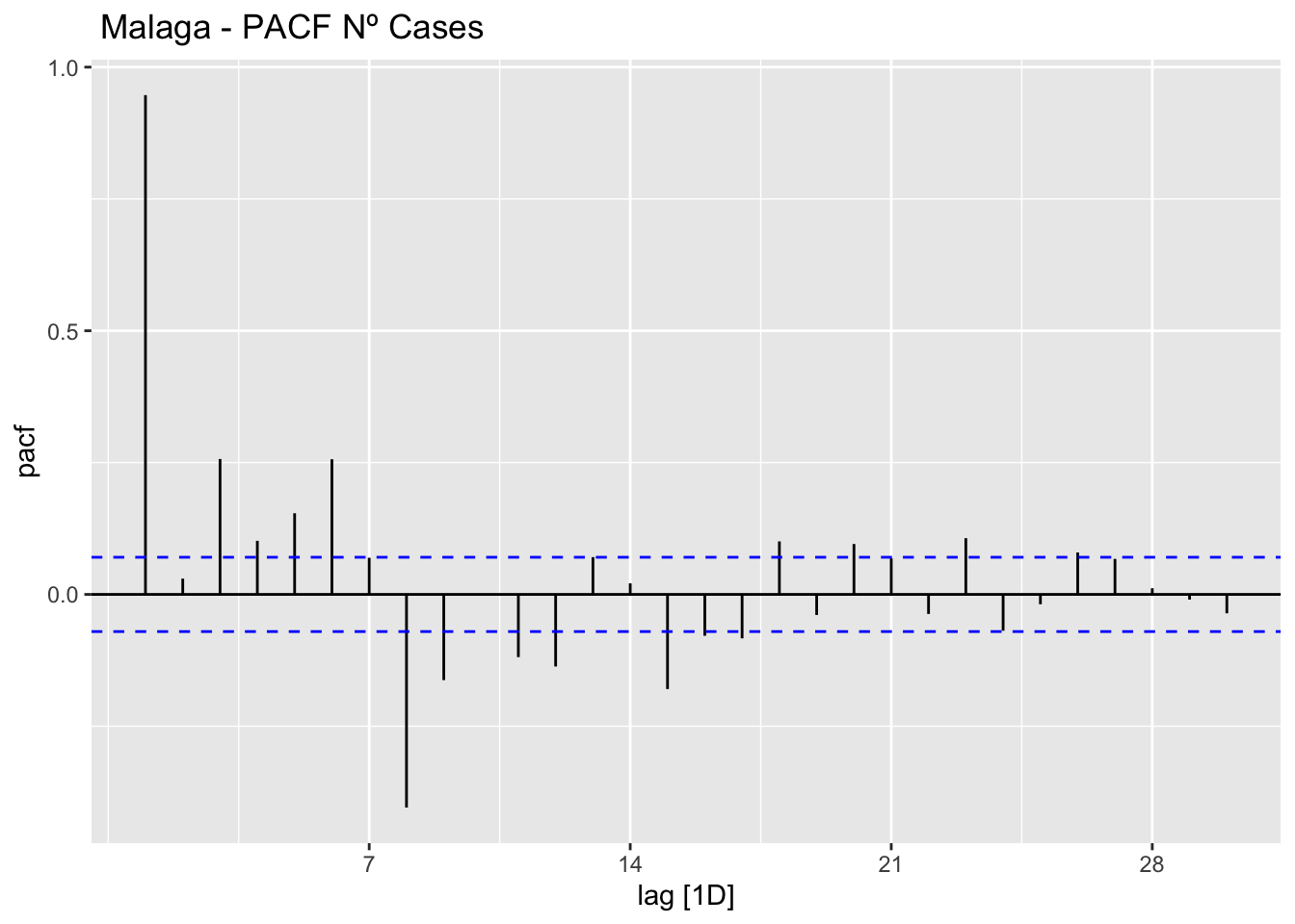
Sevilla
data_sevilla <- covid_data %>%
      filter(provincia == "Sevilla") %>%
      select(provincia, fecha, num_casos, num_hosp, tmed, mob_grocery_pharmacy, mob_parks,
             mob_residential, mob_retail_recreation, mob_transit_stations, mob_workplaces, mob_flujo) %>%
      # Drop NAs dates except for mob_flujo since the data finish in 2021 while other sources are ut to 31/03/2022
      drop_na(-mob_flujo) %>%
      as_tsibble(key = provincia, index = fecha)
data_sevilla
# A tsibble: 774 x 12 [1D]
# Key: provincia [1]
provincia fecha num_casos num_hosp tmed mob_grocery_pharmacy mob_parks
<chr> <date> <dbl> <dbl> <dbl> <dbl> <dbl>
1 Sevilla 2020-02-15 0 1 15.9 -5 34
2 Sevilla 2020-02-16 0 0 15.3 1 15
3 Sevilla 2020-02-17 0 0 16.1 0 14
4 Sevilla 2020-02-18 1 1 17.4 -1 16
5 Sevilla 2020-02-19 0 1 15.9 0 14
6 Sevilla 2020-02-20 1 1 16 -1 13
7 Sevilla 2020-02-21 0 0 15.8 -1 18
8 Sevilla 2020-02-22 0 0 16.6 -2 33
9 Sevilla 2020-02-23 0 0 16.2 5 20
10 Sevilla 2020-02-24 2 0 16.3 1 23
# … with 764 more rows, and 5 more variables: mob_residential <dbl>,
# mob_retail_recreation <dbl>, mob_transit_stations <dbl>,
# mob_workplaces <dbl>, mob_flujo <dbl># ACF
data_sevilla %>%
ACF(num_casos, lag_max = 30) %>%
autoplot() +
labs(title=" Sevilla - ACF Nº Cases")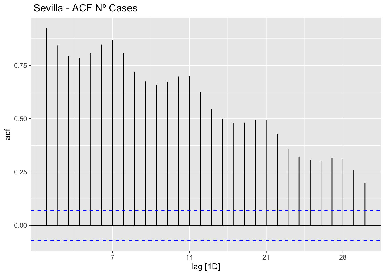
# PACF
data_sevilla %>%
      PACF(num_casos, lag_max = 30) %>%
      autoplot() +
      labs(title=" Sevilla - PACF Nº Cases")