pacman::p_load(
      here,      # file locator
      tidyverse, # data management and ggplot2 graphics
      skimr,     # get overview of data
      janitor,   # produce and adorn tabulations and cross-tabulations
      tsibble,
      fable,
      feasts
)

covid_data <- readRDS(here("data", "clean", "final_covid_data.rds"))STL decomposition / Transformations
Load packages and data:
Asturias
data_asturias <- covid_data %>%
      filter(provincia == "Asturias") %>%
      select(provincia, fecha, num_casos, num_hosp, tmed,mob_grocery_pharmacy, mob_parks,
             mob_residential, mob_retail_recreation, mob_transit_stations, mob_workplaces, mob_flujo) %>%
      # Drop NAs dates except for mob_flujo since the data finish in 2021 while other sources are ut to 31/03/2022
      drop_na(-mob_flujo) %>%
      as_tsibble(key = provincia, index = fecha)
data_asturias
# A tsibble: 774 x 12 [1D]
# Key: provincia [1]
provincia fecha num_casos num_hosp tmed mob_grocery_pharmacy mob_parks
<chr> <date> <dbl> <dbl> <dbl> <dbl> <dbl>
1 Asturias 2020-02-15 0 0 12.2 -1 20
2 Asturias 2020-02-16 0 0 16.2 1 11
3 Asturias 2020-02-17 0 2 9.8 0 -13
4 Asturias 2020-02-18 0 0 8.8 1 11
5 Asturias 2020-02-19 0 0 8.6 1 29
6 Asturias 2020-02-20 0 0 9.9 0 32
7 Asturias 2020-02-21 0 0 11.2 -1 18
8 Asturias 2020-02-22 0 0 10.5 1 29
9 Asturias 2020-02-23 1 0 9.2 6 23
10 Asturias 2020-02-24 0 0 8.6 5 48
# … with 764 more rows, and 5 more variables: mob_residential <dbl>,
# mob_retail_recreation <dbl>, mob_transit_stations <dbl>,
# mob_workplaces <dbl>, mob_flujo <dbl>data_asturias %>%
model(STL(num_casos ~ season(window = 7) + trend(window = 7))) %>%
components() %>%
autoplot() +
labs(title = "Asturias STL") +
theme_bw()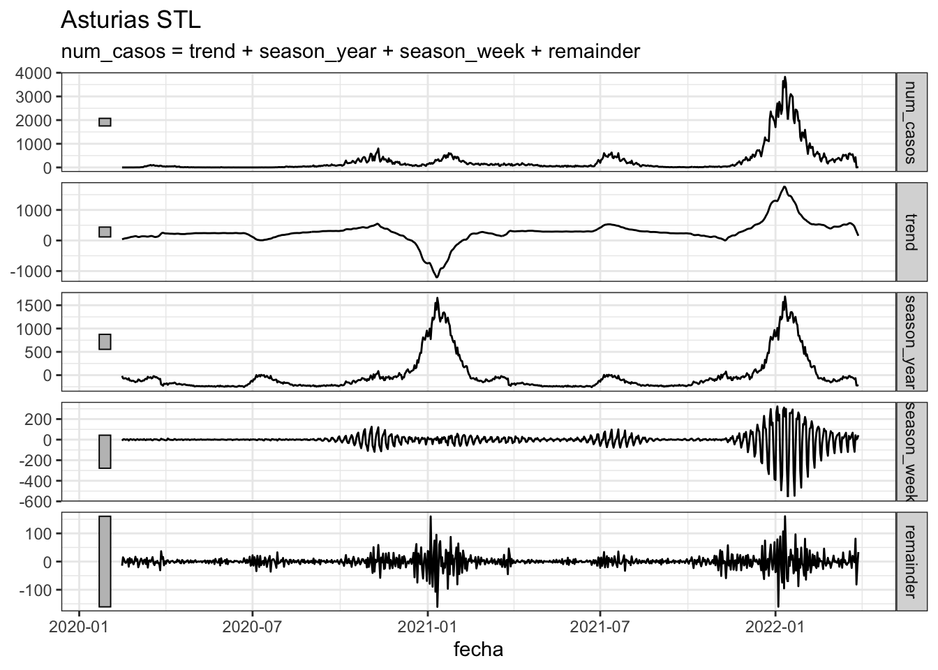
data_asturias %>%
      model(STL(num_casos ~ season(window = 7) + trend(window = 7))) %>%
      components() %>%
      as_tsibble() %>%
      autoplot(num_casos, color = "grey") +
      geom_line(aes(y = season_adjust), color = "red") +
      geom_line(aes(y = trend), color = "blue") +
      labs(title="Asturias season adjusted and trend") +
      theme_bw()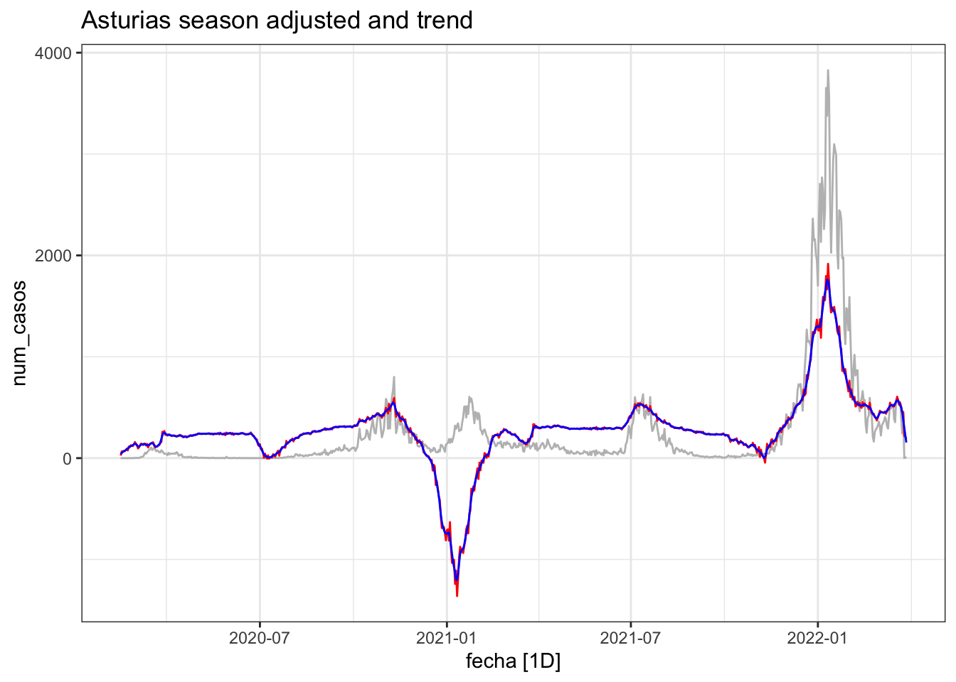
lambda_asturias <- data_asturias %>%
      features(num_casos, features = guerrero) %>%
      pull(lambda_guerrero)
lambda_asturias
[1] 0.2253939data_asturias %>%
gg_tsdisplay(
box_cox(num_casos, lambda_asturias),
plot_type = 'partial', lag = 30
) +
labs(title = "Asturias - Variance stb")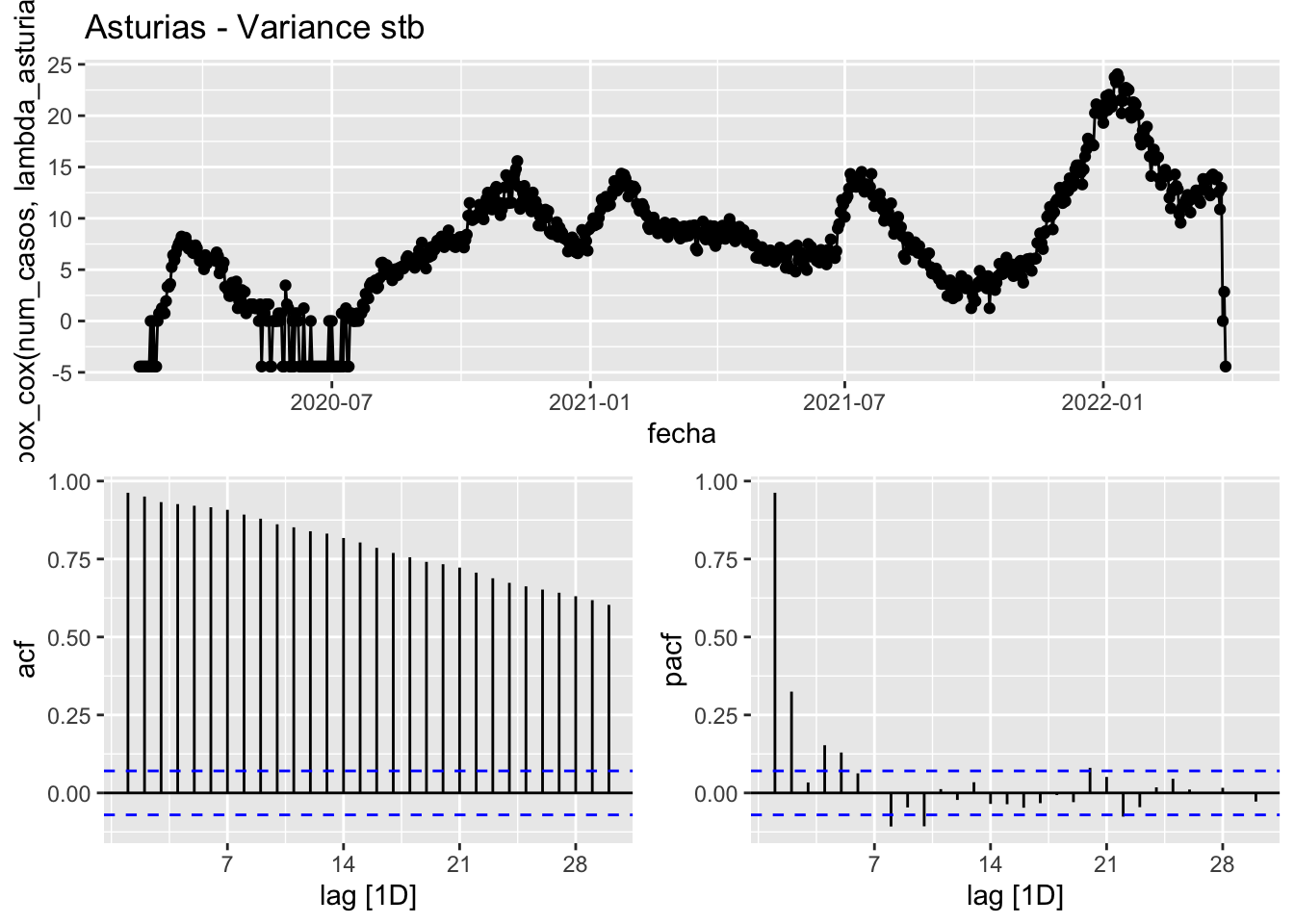
data_asturias %>%
      gg_tsdisplay(
            difference(box_cox(num_casos, lambda_asturias)),
            plot_type = 'partial', lag = 30
      ) +
      labs(title = "Asturias - Difference once")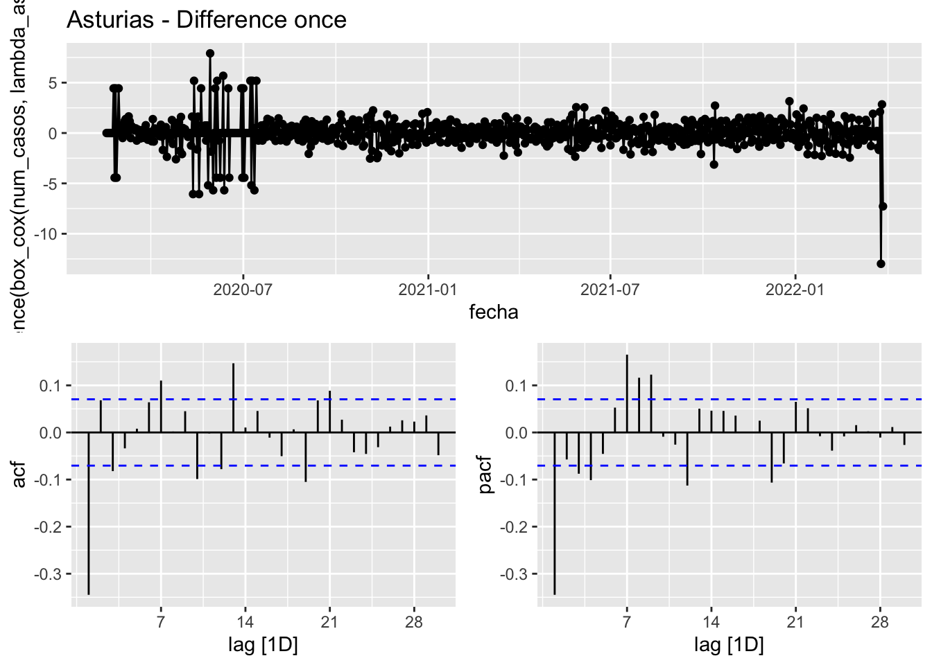
data_asturias %>%
      gg_tsdisplay(
            difference(box_cox(num_casos, lambda_asturias)) %>% difference(),
            plot_type = 'partial', lag = 30
      ) +
      labs(title="Asturias - Difference double")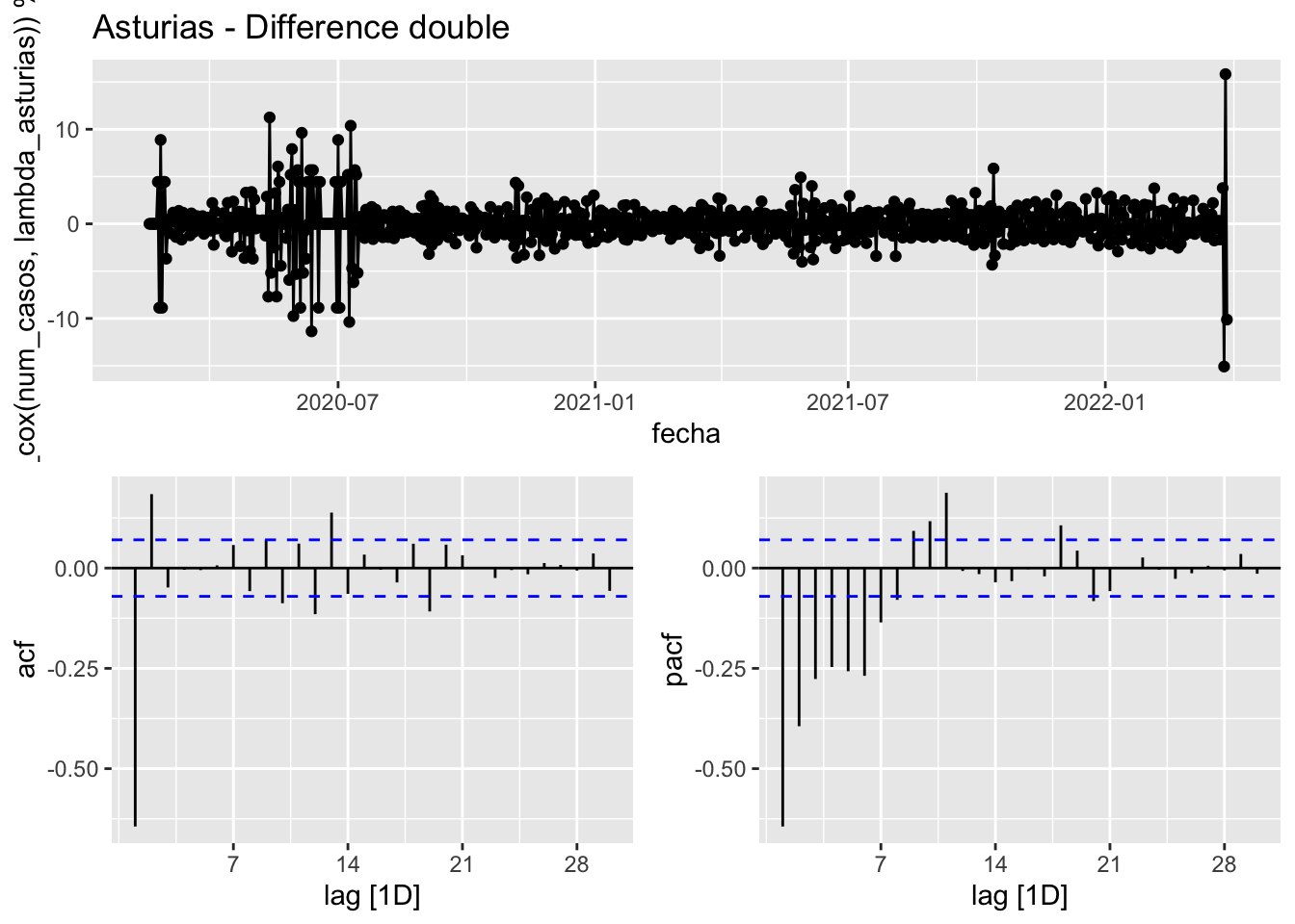
data_asturias %>%
      model(
            STL(num_casos ~ season(window = 7) + trend(window = 7),
                robust = TRUE)
      ) %>%
      components() %>%
      gg_tsdisplay(season_adjust, plot_type = 'partial', lag = 30) +
      labs(title="Asturias - Orginal STL season_adjust")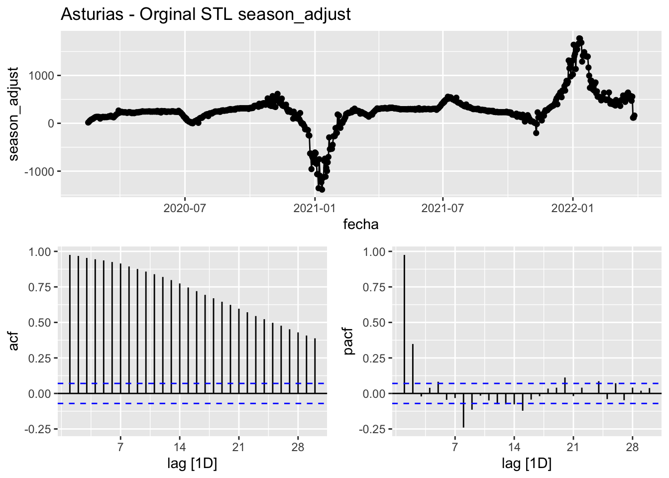
data_asturias %>%
      model(
            STL(num_casos ~ season(window = 7) + trend(window = 7),
                robust = TRUE)
      ) %>%
      components() %>%
      gg_tsdisplay(trend, plot_type = 'partial', lag = 30) +
      labs(title="Asturias - Orginal STL trend")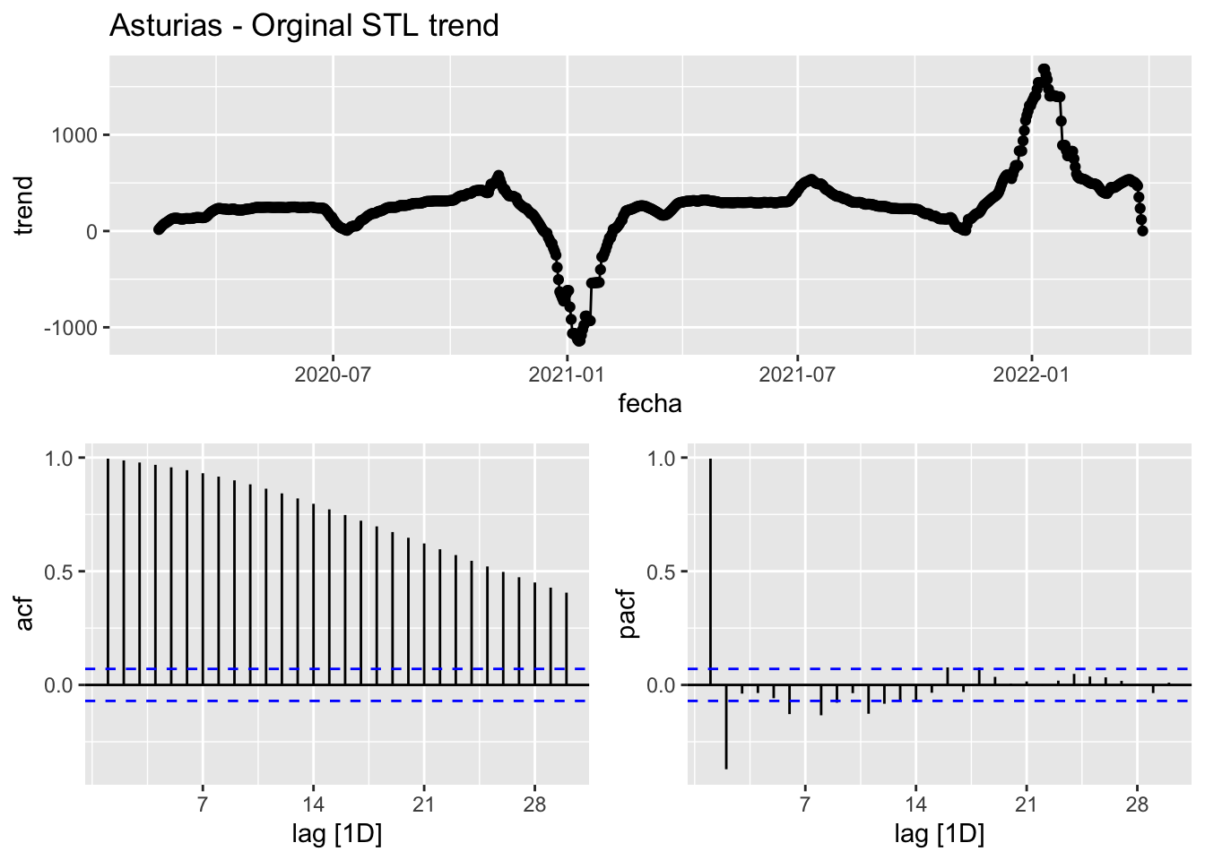
data_asturias %>%
      model(
            STL(num_casos ~ season(window = 7) + trend(window = 7),
                robust = TRUE)
      ) %>%
      components() %>%
      select(trend) %>%
      gg_tsdisplay(difference(trend), plot_type = 'partial', lag = 30) +
      labs(title="Asturias - Orginal STL trend first difference")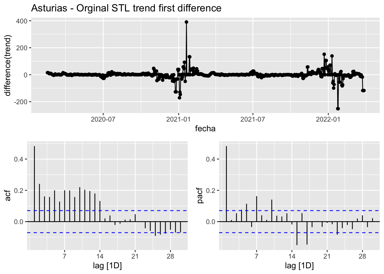
data_asturias %>%
      model(
            STL(num_casos ~ season(window = 7) + trend(window = 7),
                robust = TRUE)
      ) %>%
      components() %>%
      select(trend) %>%
      gg_tsdisplay(difference(difference(trend)), plot_type = 'partial', lag = 30) +
      labs(title="Asturias - Orginal STL trend second difference")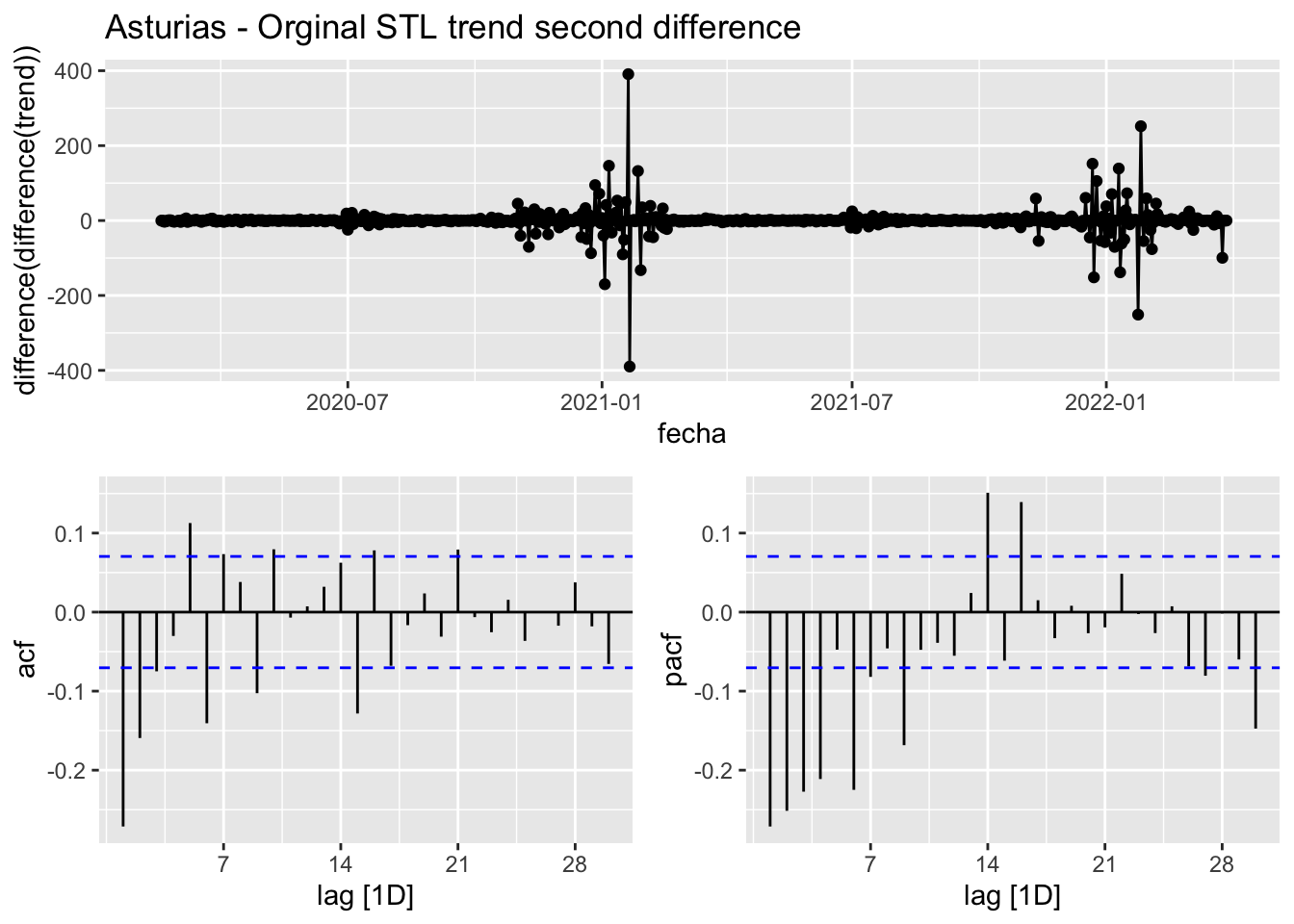
Barcelona
data_barcelona <- covid_data %>%
      filter(provincia == "Barcelona") %>%
      select(provincia, fecha, num_casos, num_hosp, tmed,mob_grocery_pharmacy, mob_parks,
             mob_residential, mob_retail_recreation, mob_transit_stations, mob_workplaces, mob_flujo) %>%
      # Drop NAs dates except for mob_flujo since the data finish in 2021 while other sources are ut to 31/03/2022
      drop_na(-mob_flujo) %>%
      as_tsibble(key = provincia, index = fecha)
data_barcelona
# A tsibble: 774 x 12 [1D]
# Key: provincia [1]
provincia fecha num_casos num_hosp tmed mob_grocery_pharmacy mob_parks
<chr> <date> <dbl> <dbl> <dbl> <dbl> <dbl>
1 Barcelona 2020-02-15 12 4 12.8 -3 14
2 Barcelona 2020-02-16 2 4 14.5 -8 2
3 Barcelona 2020-02-17 1 5 14.6 1 11
4 Barcelona 2020-02-18 5 7 11.5 1 8
5 Barcelona 2020-02-19 1 8 11.8 1 6
6 Barcelona 2020-02-20 11 10 10.4 1 9
7 Barcelona 2020-02-21 15 8 11.9 -1 11
8 Barcelona 2020-02-22 8 10 12 -1 25
9 Barcelona 2020-02-23 7 8 12.9 0 26
10 Barcelona 2020-02-24 8 4 13.6 1 21
# … with 764 more rows, and 5 more variables: mob_residential <dbl>,
# mob_retail_recreation <dbl>, mob_transit_stations <dbl>,
# mob_workplaces <dbl>, mob_flujo <dbl>data_barcelona %>%
model(STL(num_casos ~ season(window = 7) + trend(window = 7))) %>%
components() %>%
autoplot() +
labs(title = "Barcelona STL") +
theme_bw()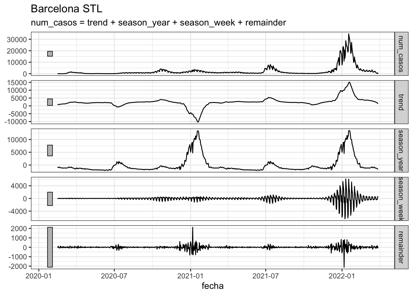
data_barcelona %>%
      model(STL(num_casos ~ season(window = 7) + trend(window = 7))) %>%
      components() %>%
      as_tsibble() %>%
      autoplot(num_casos, color = "grey") +
      geom_line(aes(y = season_adjust), color = "red") +
      geom_line(aes(y = trend), color = "blue") +
      labs(title="Barcelona season adjusted and trend") +
      theme_bw()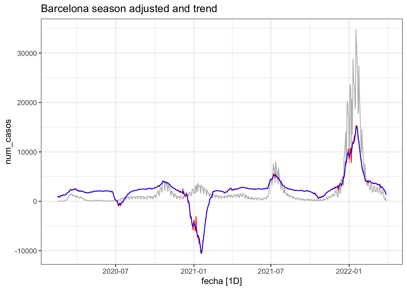
lambda_barcelona <- data_barcelona %>%
      features(num_casos, features = guerrero) %>%
      pull(lambda_guerrero)
lambda_barcelona
[1] 0.1052672data_barcelona %>%
gg_tsdisplay(
box_cox(num_casos, lambda_barcelona),
plot_type = 'partial', lag = 30
) +
labs(title = "Barcelona - Variance stb")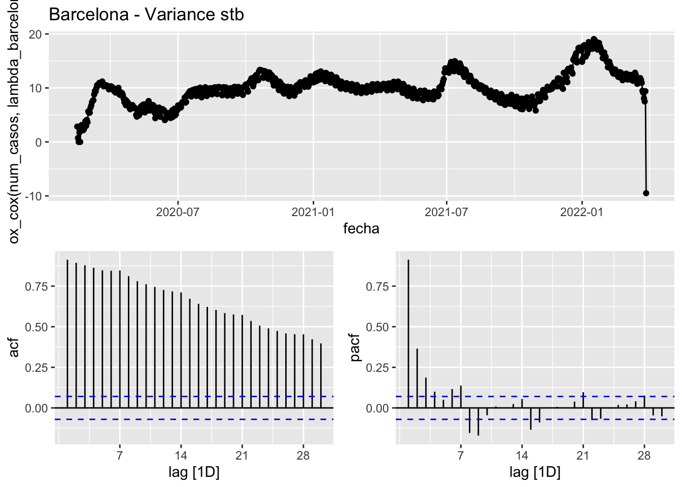
data_barcelona %>%
      gg_tsdisplay(
            difference(box_cox(num_casos, lambda_barcelona)),
            plot_type = 'partial', lag = 30
      ) +
      labs(title = "Barcelona - Difference once")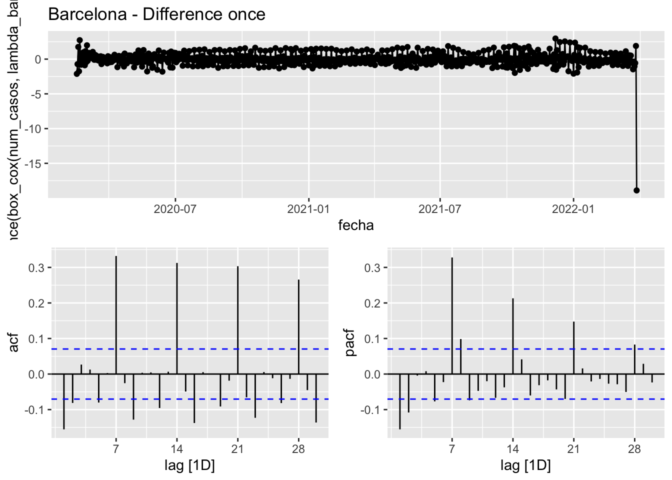
data_barcelona %>%
      gg_tsdisplay(
            difference(box_cox(num_casos, lambda_barcelona)) %>% difference(),
            plot_type = 'partial', lag = 30
      ) +
      labs(title="Barcelona - Difference double")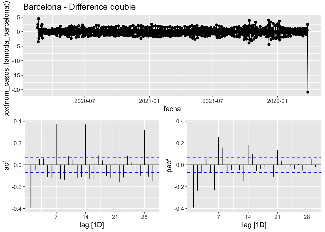
data_barcelona %>%
      model(
            STL(num_casos ~ season(window = 7) + trend(window = 7),
                robust = TRUE)
      ) %>%
      components() %>%
      gg_tsdisplay(season_adjust, plot_type = 'partial', lag = 30) +
      labs(title="Barcelona - Orginal STL season_adjust")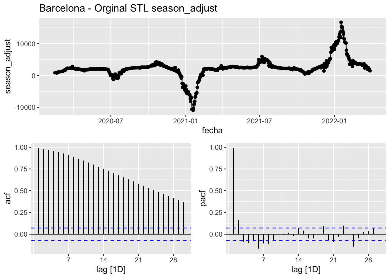
data_barcelona %>%
      model(
            STL(num_casos ~ season(window = 7) + trend(window = 7),
                robust = TRUE)
      ) %>%
      components() %>%
      gg_tsdisplay(trend, plot_type = 'partial', lag = 30) +
      labs(title="Barcelona - Orginal STL trend")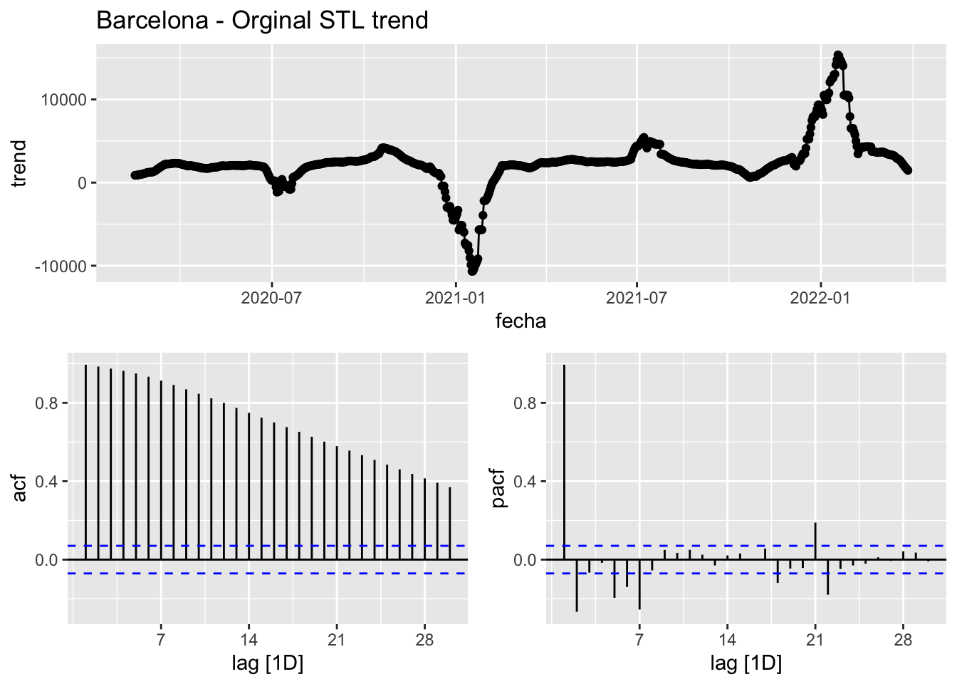
data_barcelona %>%
      model(
            STL(num_casos ~ season(window = 7) + trend(window = 7),
                robust = TRUE)
      ) %>%
      components() %>%
      gg_tsdisplay(difference(trend), plot_type = 'partial', lag = 30) +
      labs(title="Barcelona - Orginal STL trend first difference")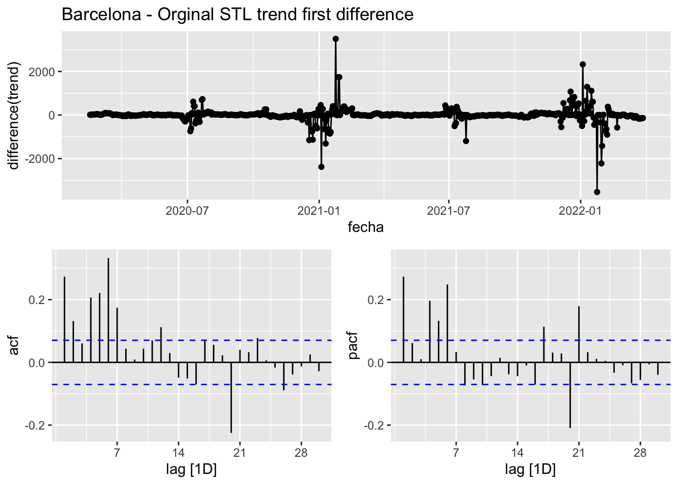
data_barcelona %>%
      model(
            STL(num_casos ~ season(window = 7) + trend(window = 7),
                robust = TRUE)
      ) %>%
      components() %>%
      gg_tsdisplay(difference(difference(trend)), plot_type = 'partial', lag = 30) +
      labs(title="Barcelona - Orginal STL trend second difference")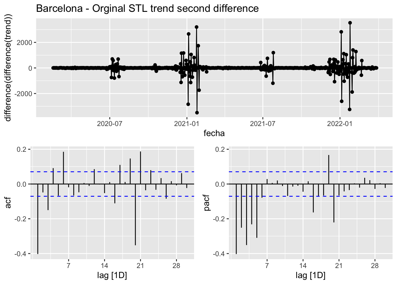
Madrid
data_madrid <- covid_data %>%
      filter(provincia == "Madrid") %>%
      select(provincia, fecha, num_casos, num_hosp, tmed,mob_grocery_pharmacy, mob_parks,
             mob_residential, mob_retail_recreation, mob_transit_stations, mob_workplaces, mob_flujo) %>%
      # Drop NAs dates except for mob_flujo since the data finish in 2021 while other sources are ut to 31/03/2022
      drop_na(-mob_flujo) %>%
      as_tsibble(key = provincia, index = fecha)
data_madrid
# A tsibble: 774 x 12 [1D]
# Key: provincia [1]
provincia fecha num_casos num_hosp tmed mob_grocery_pharmacy mob_parks
<chr> <date> <dbl> <dbl> <dbl> <dbl> <dbl>
1 Madrid 2020-02-15 13 4 8.6 -2 31
2 Madrid 2020-02-16 13 2 9.6 4 34
3 Madrid 2020-02-17 19 9 9.1 3 10
4 Madrid 2020-02-18 14 13 8.5 1 11
5 Madrid 2020-02-19 12 14 8.6 1 18
6 Madrid 2020-02-20 25 15 8 1 18
7 Madrid 2020-02-21 26 18 10.4 1 22
8 Madrid 2020-02-22 29 8 10.8 -1 53
9 Madrid 2020-02-23 44 8 11.6 6 56
10 Madrid 2020-02-24 56 18 10.8 6 35
# … with 764 more rows, and 5 more variables: mob_residential <dbl>,
# mob_retail_recreation <dbl>, mob_transit_stations <dbl>,
# mob_workplaces <dbl>, mob_flujo <dbl>data_madrid %>%
model(STL(num_casos ~ season(window = 7) + trend(window = 7))) %>%
components() %>%
autoplot() +
labs(title = "Madrid STL") +
theme_bw()
data_madrid %>%
      model(STL(num_casos ~ season(window = 7) + trend(window = 7))) %>%
      components() %>%
      as_tsibble() %>%
      autoplot(num_casos, color = "grey") +
      geom_line(aes(y = season_adjust), color = "red") +
      geom_line(aes(y = trend), color = "blue") +
      labs(title="Madrid season adjusted and trend") +
      theme_bw()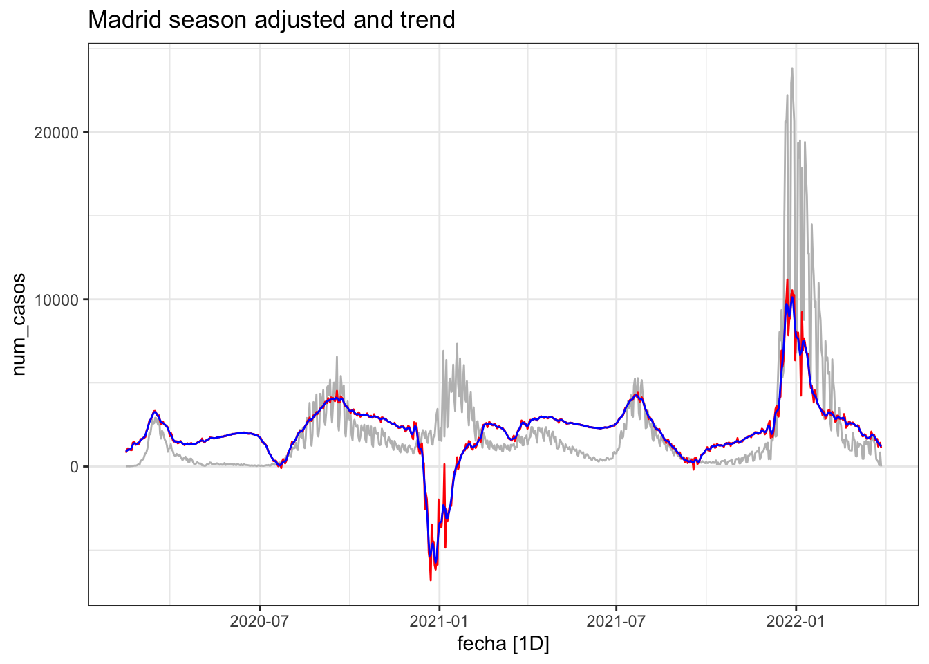
lambda_madrid <- data_madrid %>%
      features(num_casos, features = guerrero) %>%
      pull(lambda_guerrero)
lambda_madrid
[1] 0.04702742data_madrid %>%
gg_tsdisplay(
box_cox(num_casos, lambda_madrid),
plot_type = 'partial', lag = 30
) +
labs(title = "Madrid - Variance stb")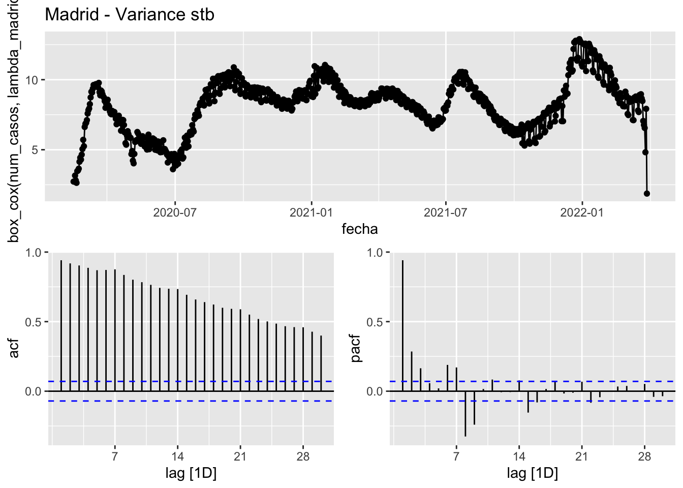
data_madrid %>%
      gg_tsdisplay(
            difference(box_cox(num_casos, lambda_madrid)),
            plot_type = 'partial', lag = 30
      ) +
      labs(title = "Madrid - Difference once")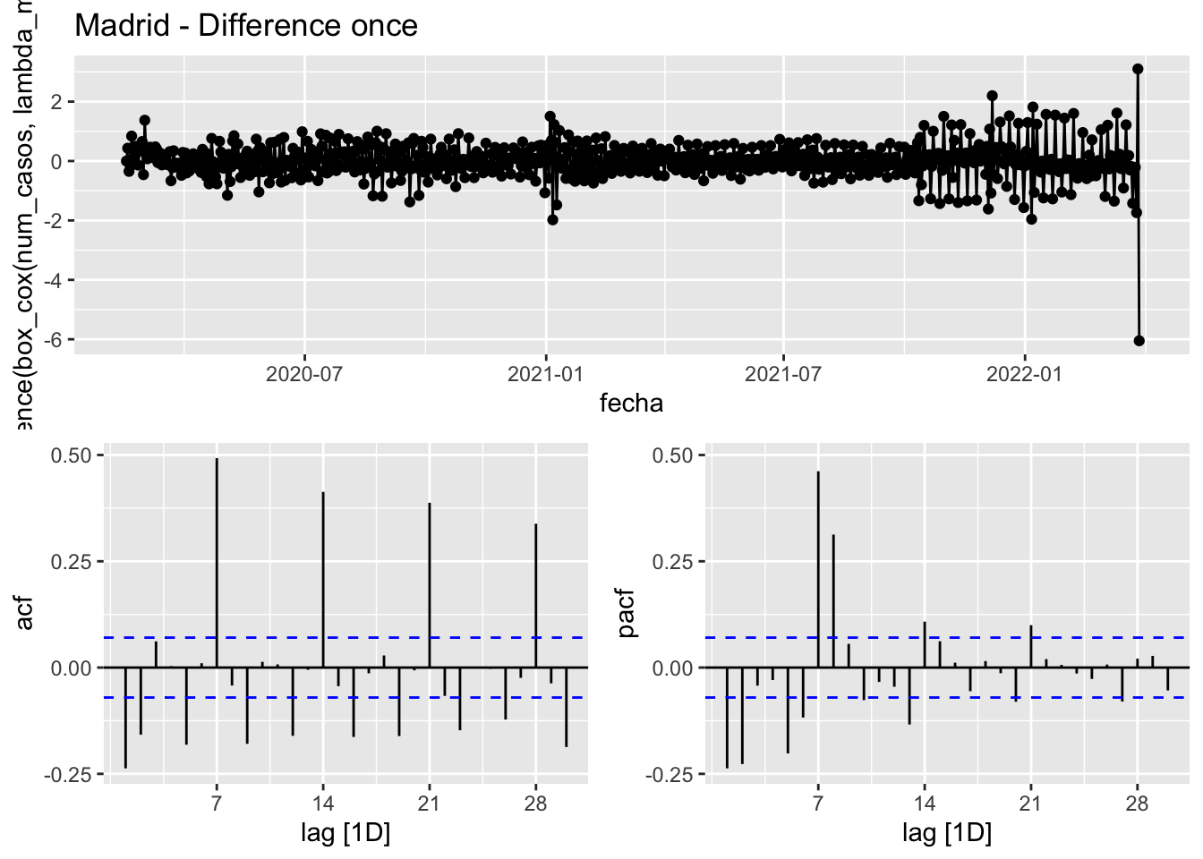
data_madrid %>%
      gg_tsdisplay(
            difference(box_cox(num_casos, lambda_madrid)) %>% difference(),
            plot_type = 'partial', lag = 30
      ) +
      labs(title="Madrid - Difference double")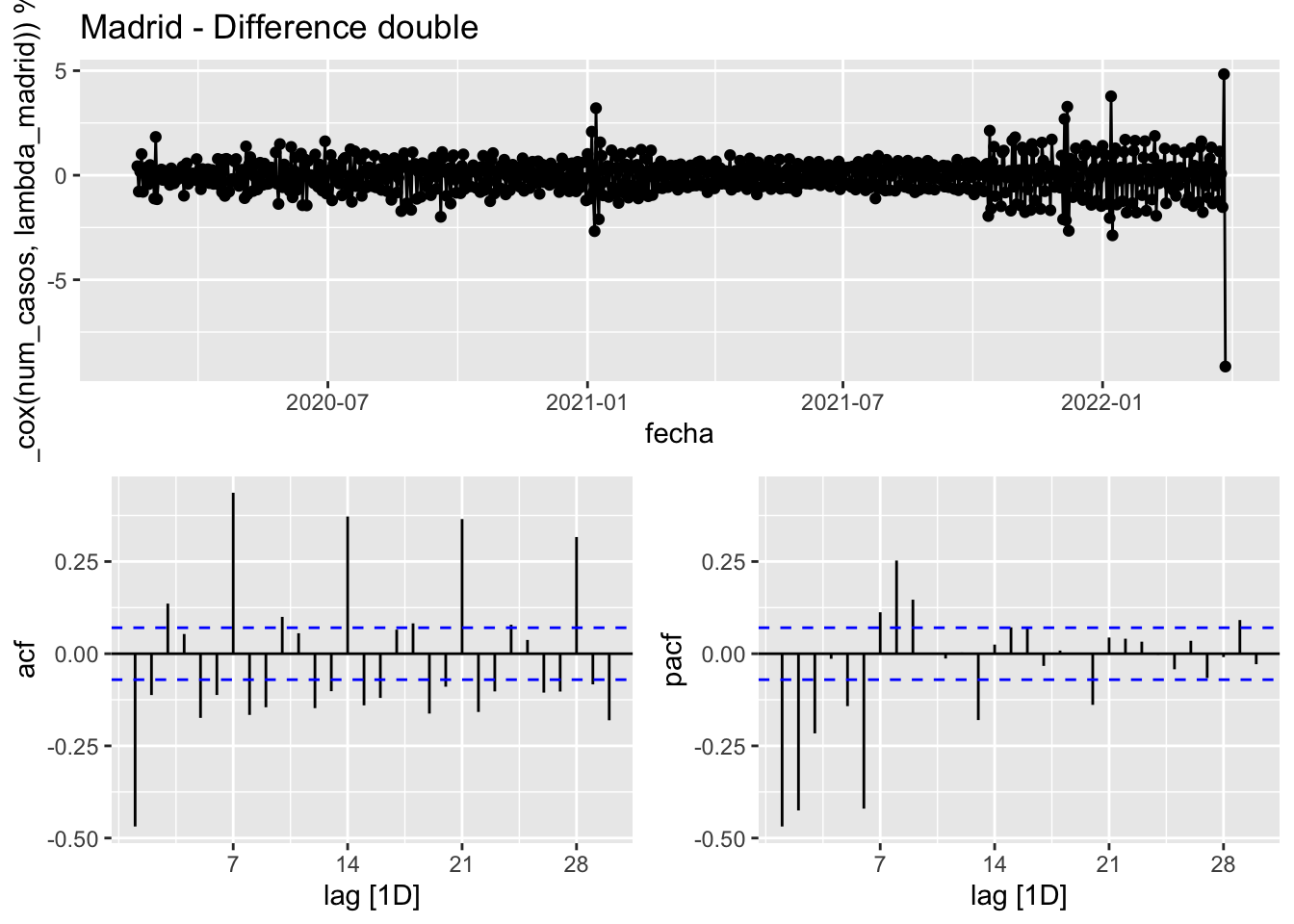
data_madrid %>%
      model(
            STL(num_casos ~ season(window = 7) + trend(window = 7),
                robust = TRUE)
      ) %>%
      components() %>%
      gg_tsdisplay(season_adjust, plot_type = 'partial', lag = 30) +
      labs(title="Madrid - Orginal STL season_adjust")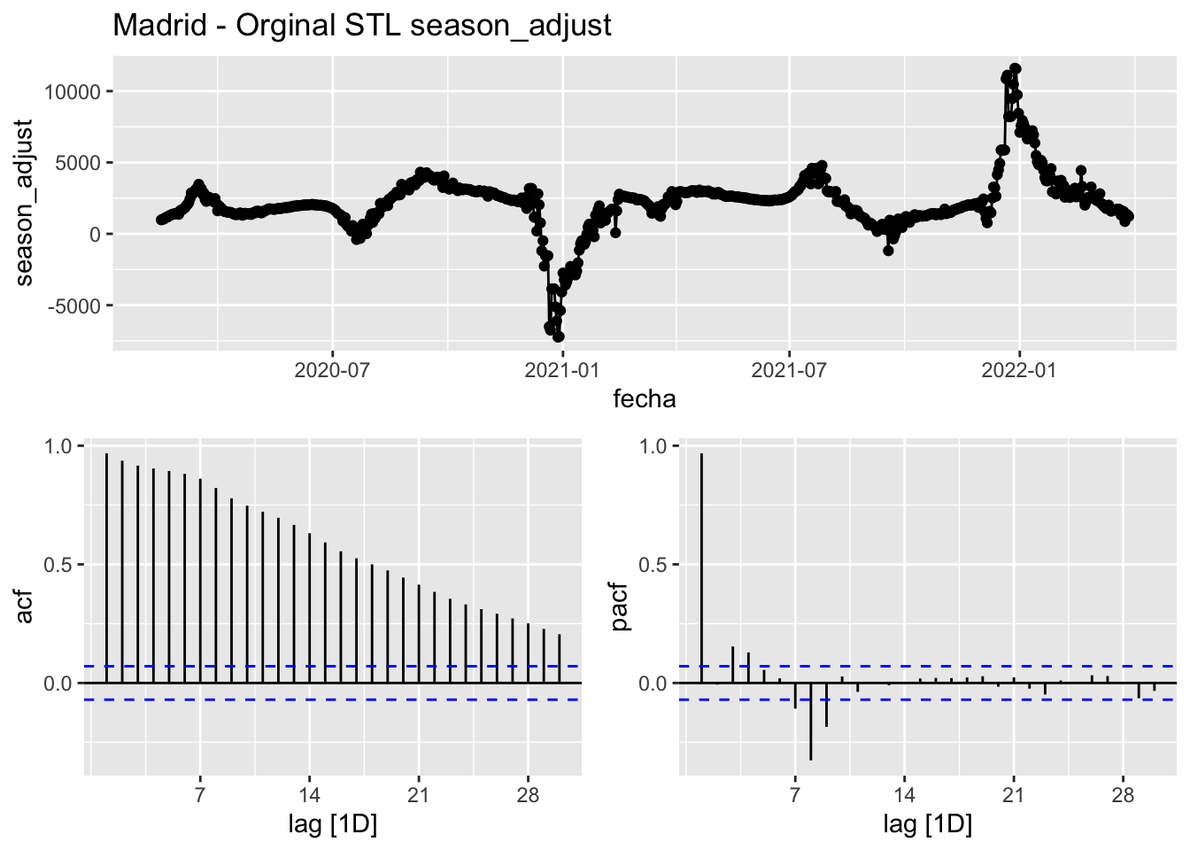
data_madrid %>%
      model(
            STL(num_casos ~ season(window = 7) + trend(window = 7),
                robust = TRUE)
      ) %>%
      components() %>%
      gg_tsdisplay(trend, plot_type = 'partial', lag = 30) +
      labs(title="Madrid - Orginal STL trend")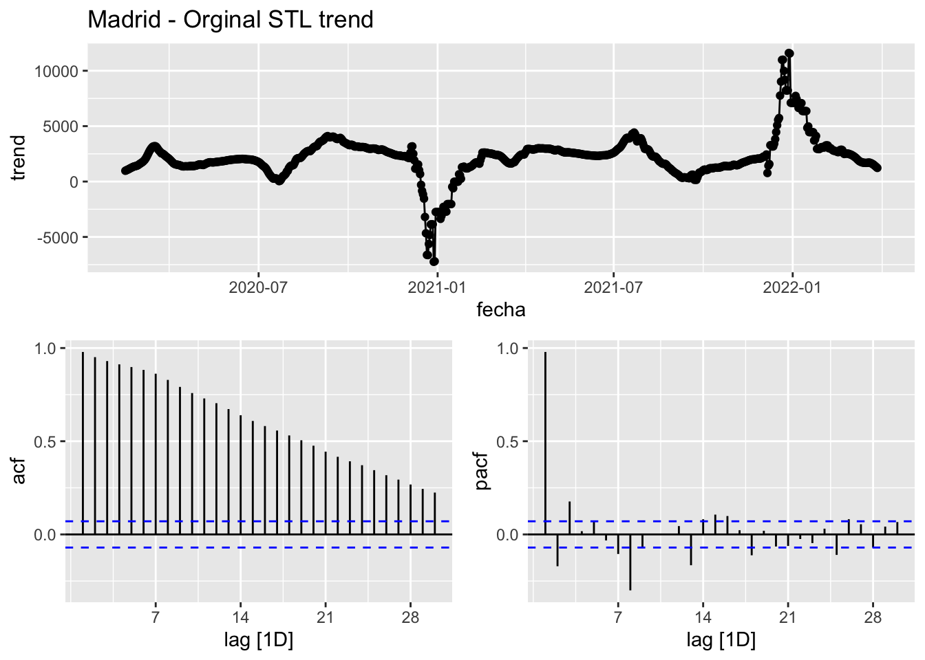
data_madrid %>%
      model(
            STL(num_casos ~ season(window = 7) + trend(window = 7),
                robust = TRUE)
      ) %>%
      components() %>%
      gg_tsdisplay(difference(trend), plot_type = 'partial', lag = 30) +
      labs(title="Madrid - Orginal STL trend first difference")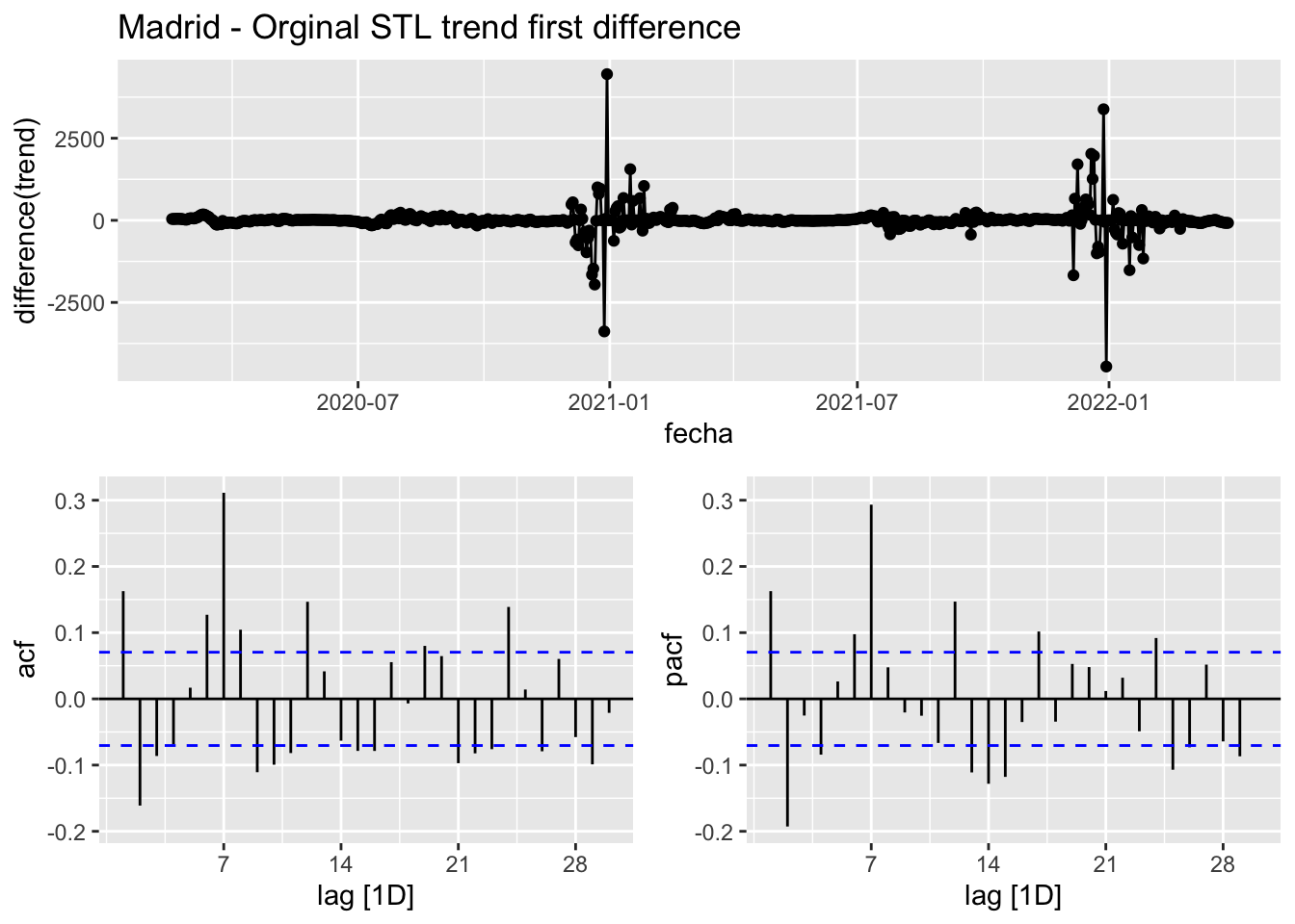
data_madrid %>%
      model(
            STL(num_casos ~ season(window = 7) + trend(window = 7),
                robust = TRUE)
      ) %>%
      components() %>%
      gg_tsdisplay(difference(difference(trend)), plot_type = 'partial', lag = 30) +
      labs(title="Madrid - Orginal STL trend second difference")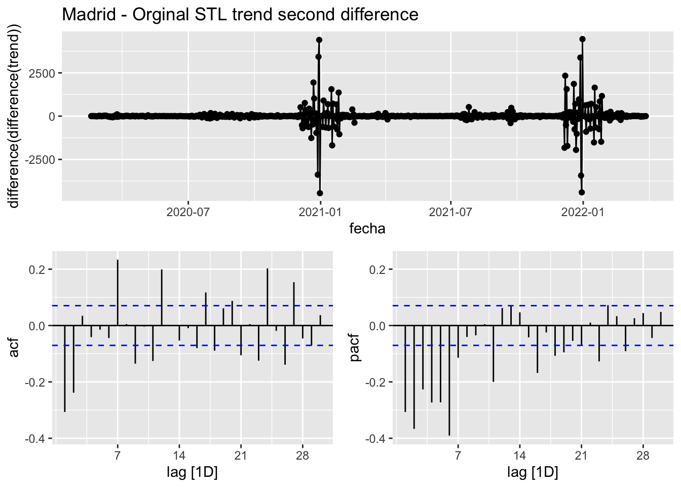
Malaga
data_malaga <- covid_data %>%
      filter(provincia == "Málaga") %>%
      select(provincia, fecha, num_casos, num_hosp, tmed,mob_grocery_pharmacy, mob_parks,
             mob_residential, mob_retail_recreation, mob_transit_stations, mob_workplaces, mob_flujo) %>%
      # Drop NAs dates except for mob_flujo since the data finish in 2021 while other sources are ut to 31/03/2022
      drop_na(-mob_flujo) %>%
      as_tsibble(key = provincia, index = fecha)
data_malaga
# A tsibble: 774 x 12 [1D]
# Key: provincia [1]
provincia fecha num_casos num_hosp tmed mob_grocery_pharmacy mob_parks
<chr> <date> <dbl> <dbl> <dbl> <dbl> <dbl>
1 Málaga 2020-02-15 1 0 13.5 0 29
2 Málaga 2020-02-16 0 0 14 4 16
3 Málaga 2020-02-17 0 0 17.1 1 14
4 Málaga 2020-02-18 0 0 15.4 0 -1
5 Málaga 2020-02-19 0 2 15.9 0 -1
6 Málaga 2020-02-20 1 0 14.9 1 13
7 Málaga 2020-02-21 3 2 13.6 -1 3
8 Málaga 2020-02-22 2 1 14.2 -1 25
9 Málaga 2020-02-23 2 0 13.2 10 15
10 Málaga 2020-02-24 2 1 14 0 22
# … with 764 more rows, and 5 more variables: mob_residential <dbl>,
# mob_retail_recreation <dbl>, mob_transit_stations <dbl>,
# mob_workplaces <dbl>, mob_flujo <dbl>data_malaga %>%
model(STL(num_casos ~ season(window = 7) + trend(window = 7))) %>%
components() %>%
autoplot() +
labs(title = "Málaga STL") +
theme_bw()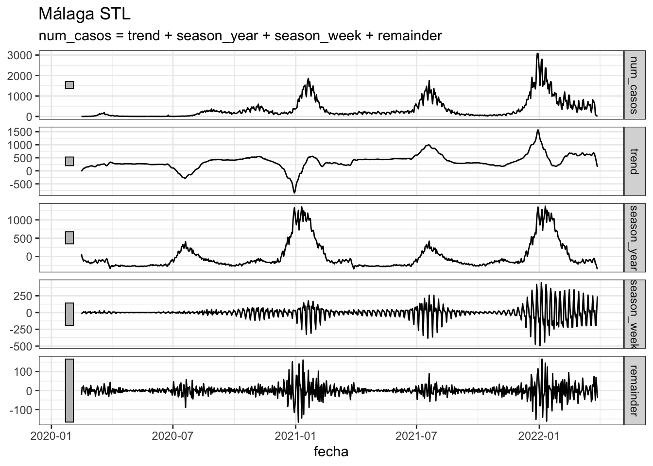
data_malaga %>%
      model(STL(num_casos ~ season(window = 7) + trend(window = 7))) %>%
      components() %>%
      as_tsibble() %>%
      autoplot(num_casos, color = "grey") +
      geom_line(aes(y = season_adjust), color = "red") +
      geom_line(aes(y = trend), color = "blue") +
      labs(title="Málaga season adjusted and trend") +
      theme_bw()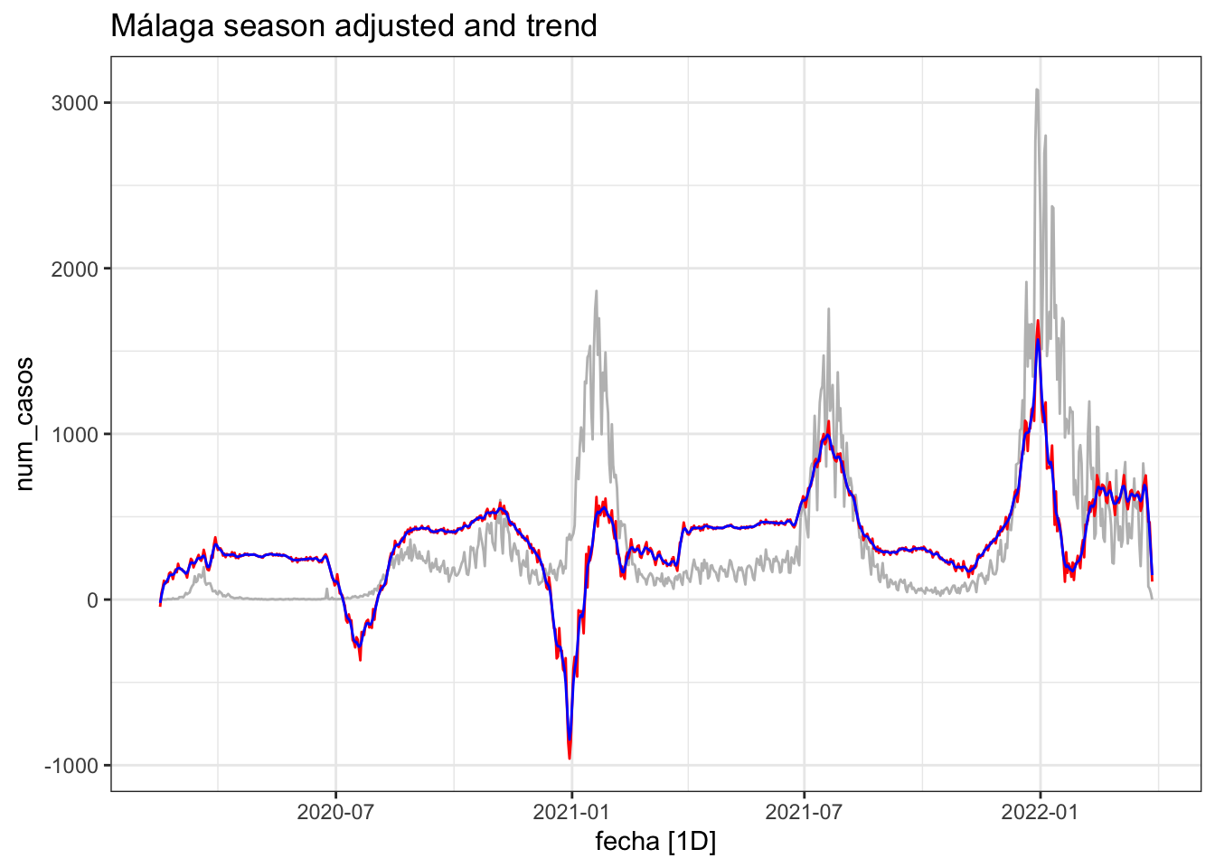
lambda_malaga <- data_malaga %>%
      features(num_casos, features = guerrero) %>%
      pull(lambda_guerrero)
lambda_malaga
[1] 0.2118375data_malaga %>%
gg_tsdisplay(
box_cox(num_casos, lambda_malaga),
plot_type = 'partial', lag = 30
) +
labs(title = "Málaga - Variance stb")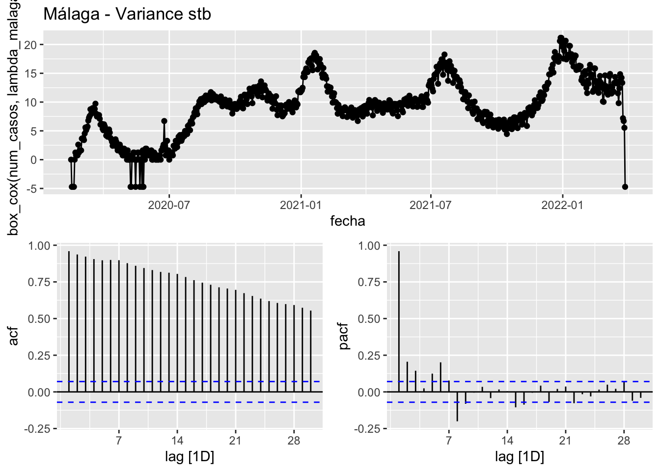
data_malaga %>%
      gg_tsdisplay(
            difference(box_cox(num_casos, lambda_malaga)),
            plot_type = 'partial', lag = 30
      ) +
      labs(title = "Málaga - Difference once")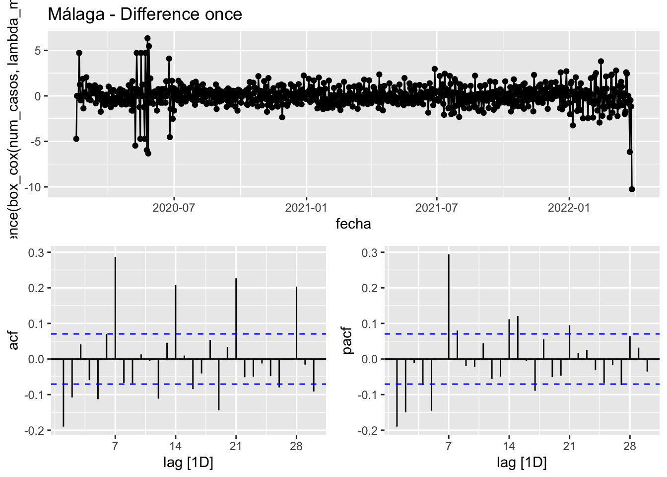
data_malaga %>%
      gg_tsdisplay(
            difference(box_cox(num_casos, lambda_malaga)) %>% difference(),
            plot_type = 'partial', lag = 30
      ) +
      labs(title="Málaga - Difference double")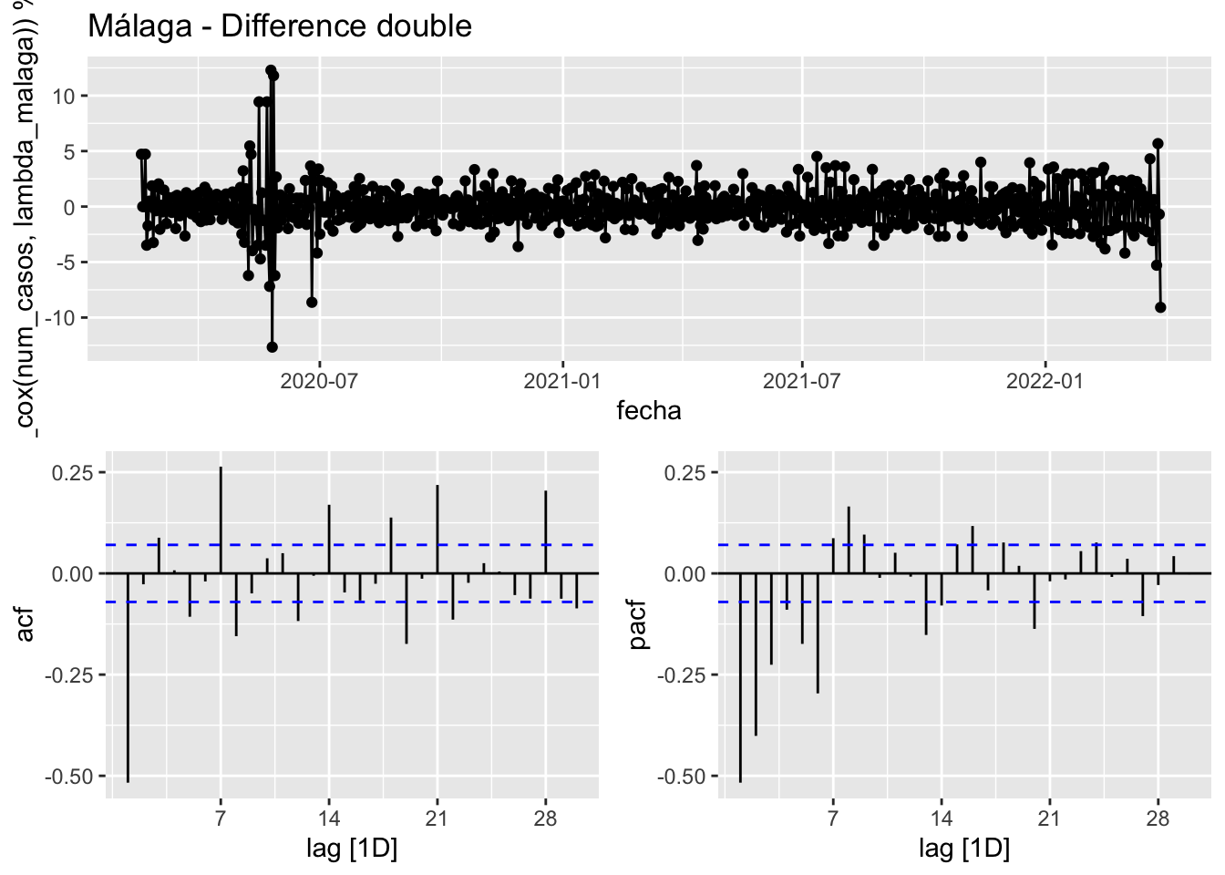
data_malaga %>%
      model(
            STL(num_casos ~ season(window = 7) + trend(window = 7),
                robust = TRUE)
      ) %>%
      components() %>%
      gg_tsdisplay(season_adjust, plot_type = 'partial', lag = 30) +
      labs(title="Málaga - Orginal STL season_adjust")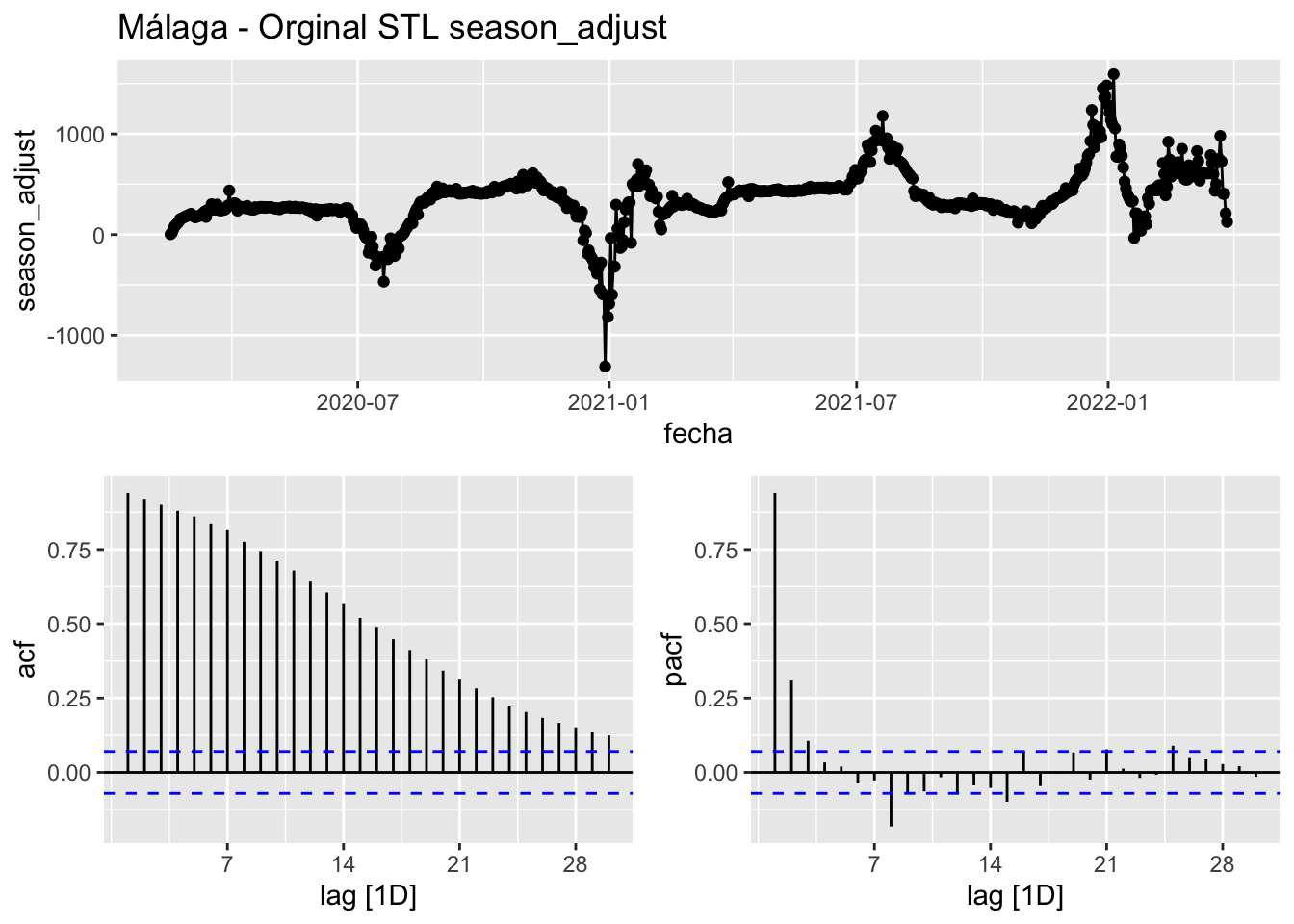
data_malaga %>%
      model(
            STL(num_casos ~ season(window = 7) + trend(window = 7),
                robust = TRUE)
      ) %>%
      components() %>%
      gg_tsdisplay(trend, plot_type = 'partial', lag = 30) +
      labs(title="Málaga - Orginal STL trend")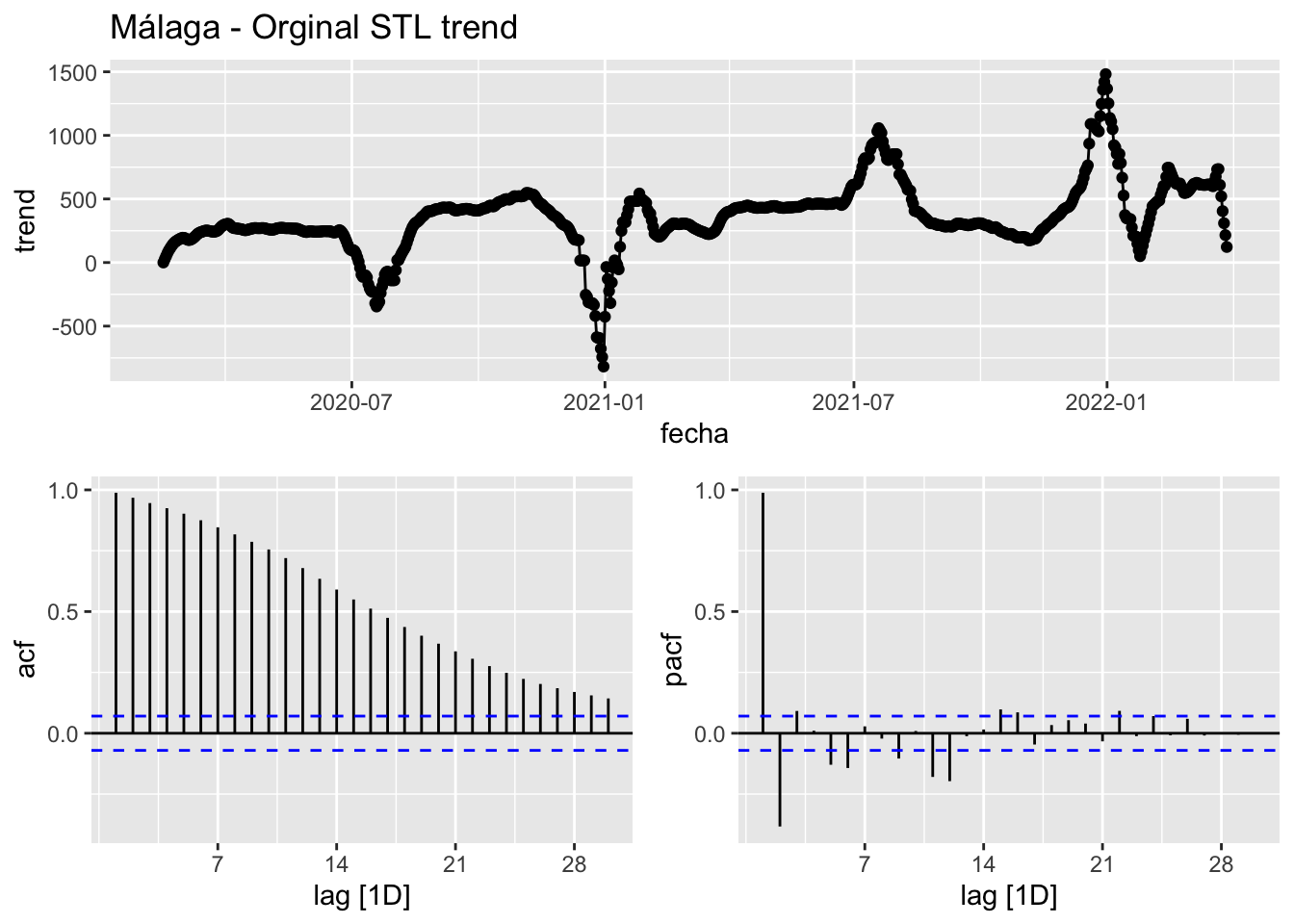
data_malaga %>%
      model(
            STL(num_casos ~ season(window = 7) + trend(window = 7),
                robust = TRUE)
      ) %>%
      components() %>%
      gg_tsdisplay(difference(trend), plot_type = 'partial', lag = 30) +
      labs(title="Málaga - Orginal STL trend first difference")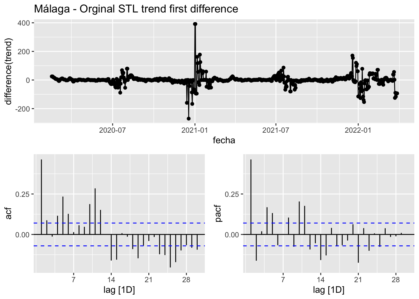
data_malaga %>%
      model(
            STL(num_casos ~ season(window = 7) + trend(window = 7),
                robust = TRUE)
      ) %>%
      components() %>%
      gg_tsdisplay(difference(difference(trend)), plot_type = 'partial', lag = 30) +
      labs(title="Málaga - Orginal STL trend second difference")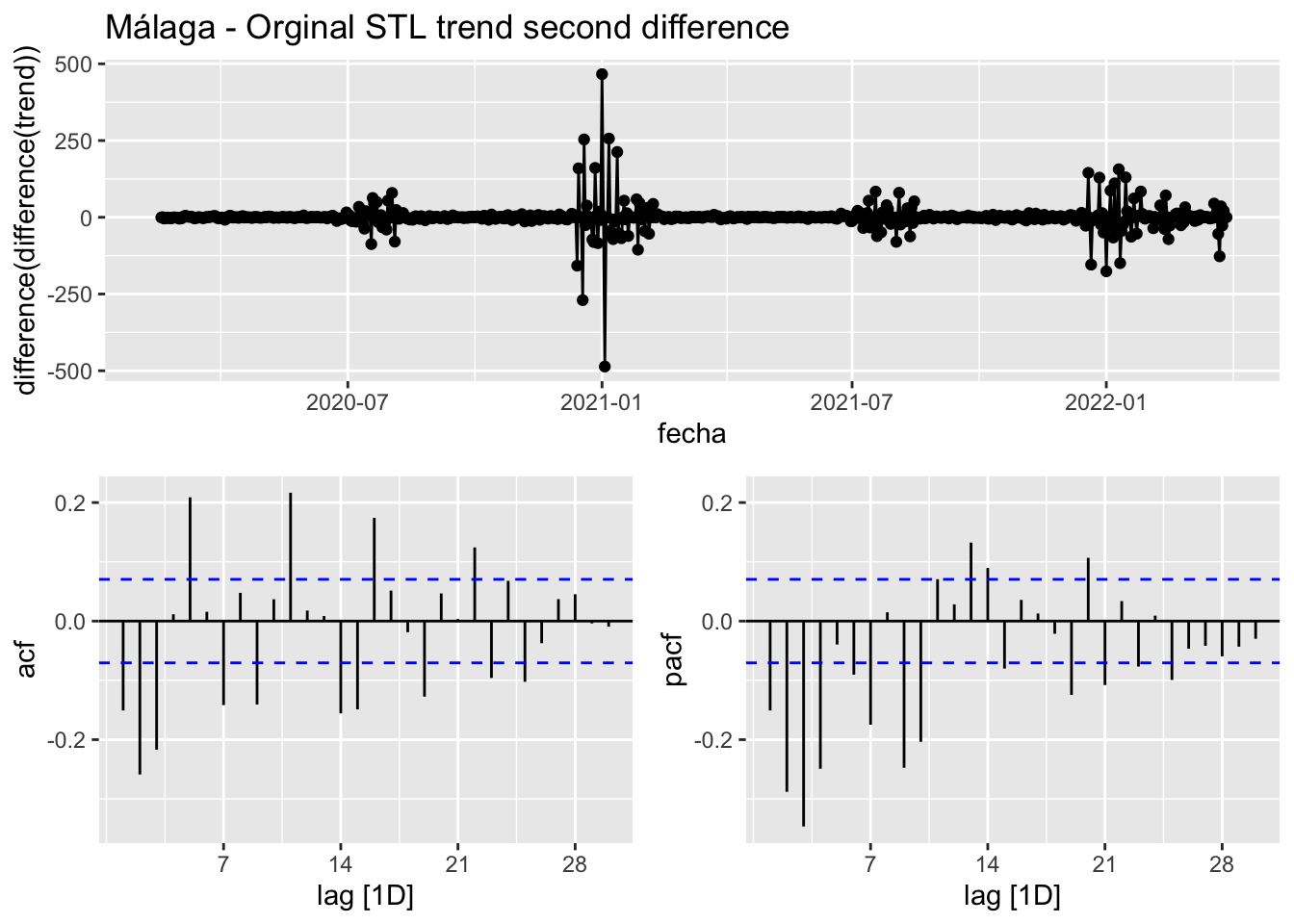
Sevilla
data_sevilla <- covid_data %>%
      filter(provincia == "Sevilla") %>%
      select(provincia, fecha, num_casos, num_hosp, tmed,mob_grocery_pharmacy, mob_parks,
             mob_residential, mob_retail_recreation, mob_transit_stations, mob_workplaces, mob_flujo) %>%
      # Drop NAs dates except for mob_flujo since the data finish in 2021 while other sources are ut to 31/03/2022
      drop_na(-mob_flujo) %>%
      as_tsibble(key = provincia, index = fecha)
data_sevilla
# A tsibble: 774 x 12 [1D]
# Key: provincia [1]
provincia fecha num_casos num_hosp tmed mob_grocery_pharmacy mob_parks
<chr> <date> <dbl> <dbl> <dbl> <dbl> <dbl>
1 Sevilla 2020-02-15 0 1 15.9 -5 34
2 Sevilla 2020-02-16 0 0 15.3 1 15
3 Sevilla 2020-02-17 0 0 16.1 0 14
4 Sevilla 2020-02-18 1 1 17.4 -1 16
5 Sevilla 2020-02-19 0 1 15.9 0 14
6 Sevilla 2020-02-20 1 1 16 -1 13
7 Sevilla 2020-02-21 0 0 15.8 -1 18
8 Sevilla 2020-02-22 0 0 16.6 -2 33
9 Sevilla 2020-02-23 0 0 16.2 5 20
10 Sevilla 2020-02-24 2 0 16.3 1 23
# … with 764 more rows, and 5 more variables: mob_residential <dbl>,
# mob_retail_recreation <dbl>, mob_transit_stations <dbl>,
# mob_workplaces <dbl>, mob_flujo <dbl>data_sevilla %>%
model(STL(num_casos ~ season(window = 7) + trend(window = 7))) %>%
components() %>%
autoplot() +
labs(title = "Sevilla STL") +
theme_bw()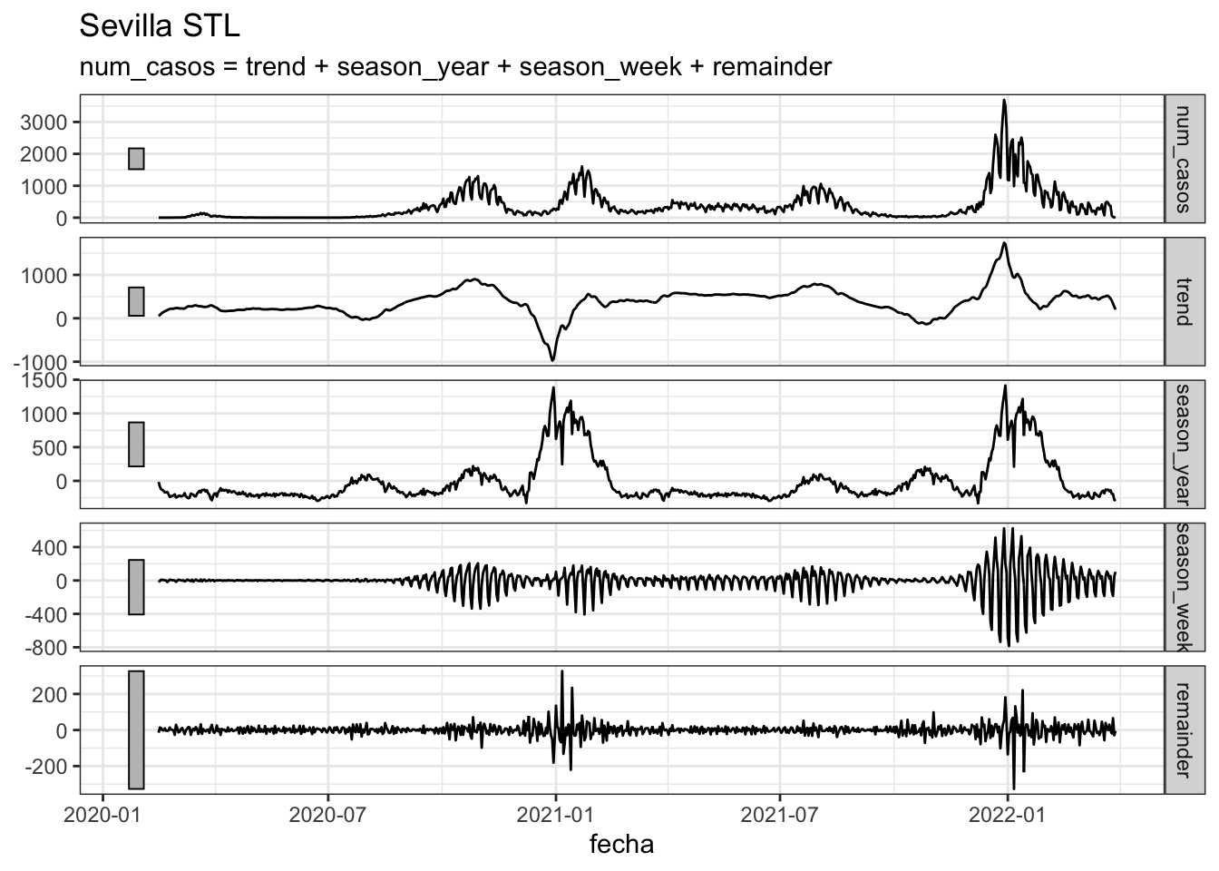
data_sevilla %>%
      model(STL(num_casos ~ season(window = 7) + trend(window = 7))) %>%
      components() %>%
      as_tsibble() %>%
      autoplot(num_casos, color = "grey") +
      geom_line(aes(y = season_adjust), color = "red") +
      geom_line(aes(y = trend), color = "blue") +
      labs(title="Sevilla season adjusted and trend") +
      theme_bw()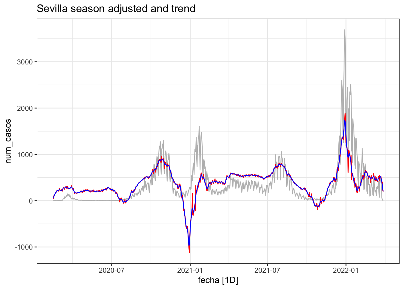
lambda_sevilla <- data_sevilla %>%
      features(num_casos, features = guerrero) %>%
      pull(lambda_guerrero)
lambda_sevilla
[1] 0.2009975data_sevilla %>%
gg_tsdisplay(
box_cox(num_casos, lambda_sevilla),
plot_type = 'partial', lag = 30
) +
labs(title = "Sevilla - Variance stb")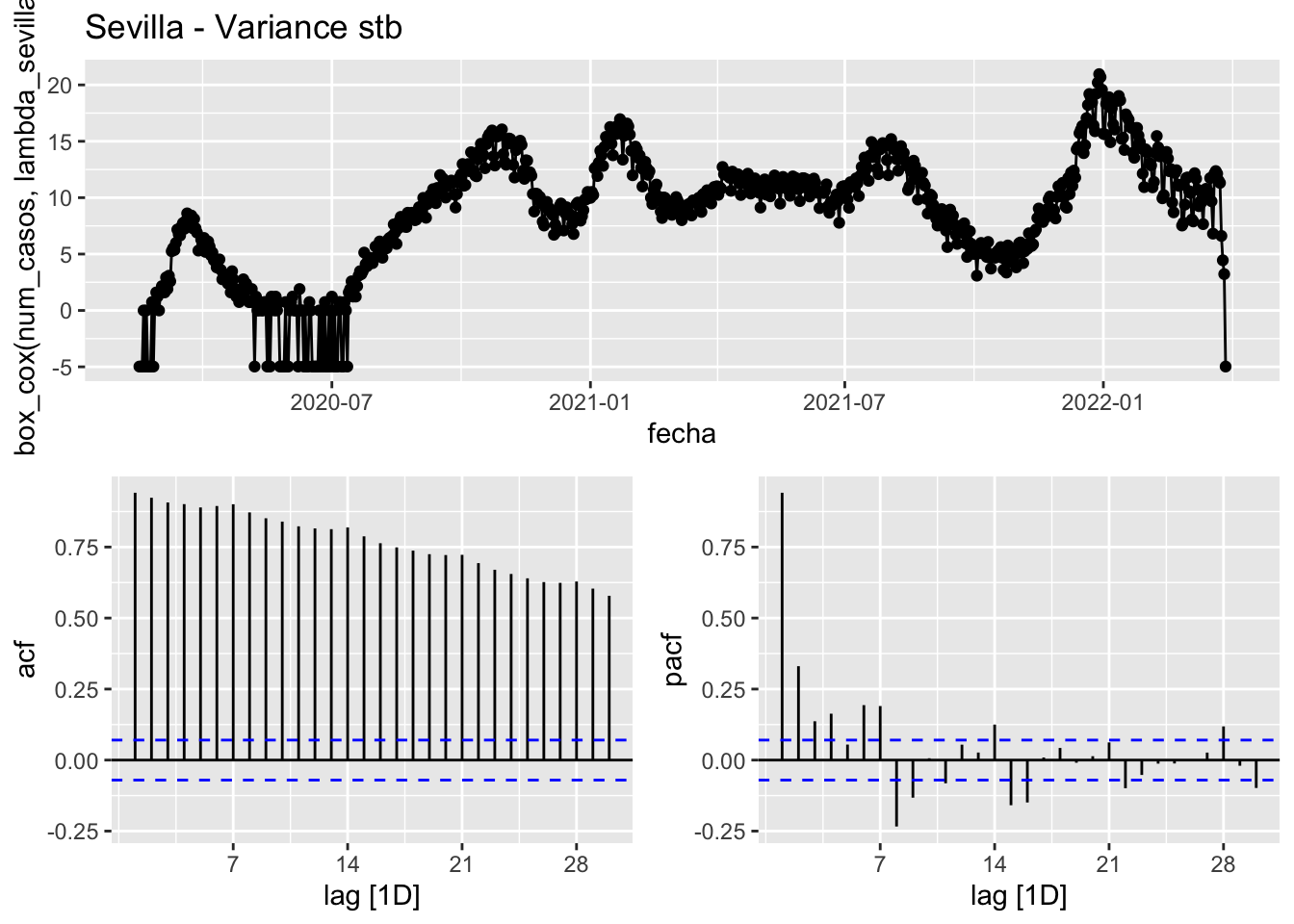
data_sevilla %>%
      gg_tsdisplay(
            difference(box_cox(num_casos, lambda_sevilla)),
            plot_type = 'partial', lag = 30
      ) +
      labs(title = "Sevilla - Difference once")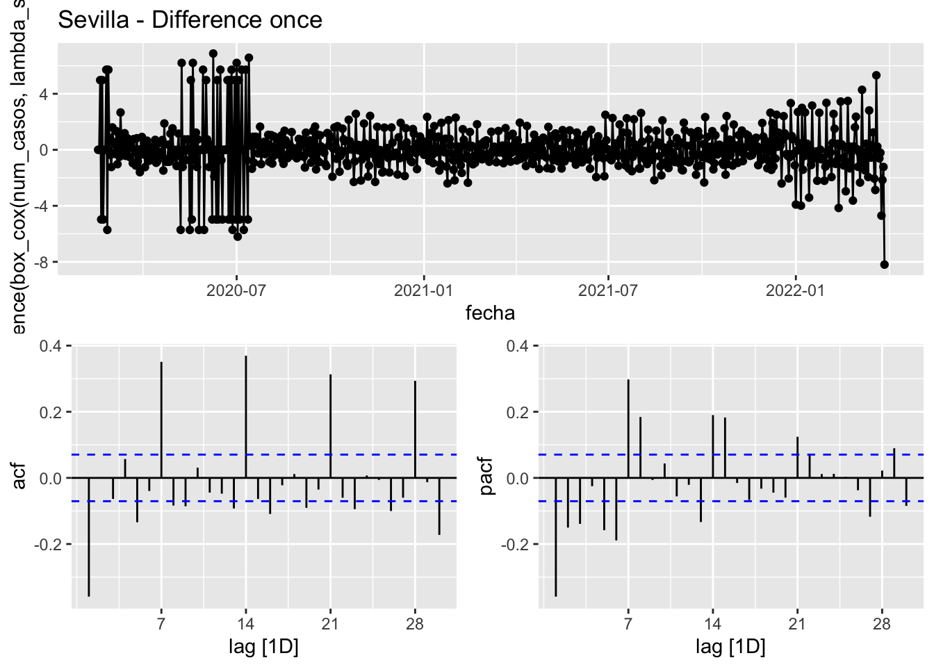
data_sevilla %>%
      gg_tsdisplay(
            difference(box_cox(num_casos, lambda_sevilla)) %>% difference(),
            plot_type = 'partial', lag = 30
      ) +
      labs(title="Sevilla - Difference double")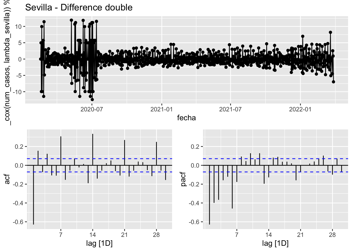
data_sevilla %>%
      model(
            STL(num_casos ~ season(window = 7) + trend(window = 7),
                robust = TRUE)
      ) %>%
      components() %>%
      gg_tsdisplay(season_adjust, plot_type = 'partial', lag = 30) +
      labs(title="Sevilla - Orginal STL season_adjust")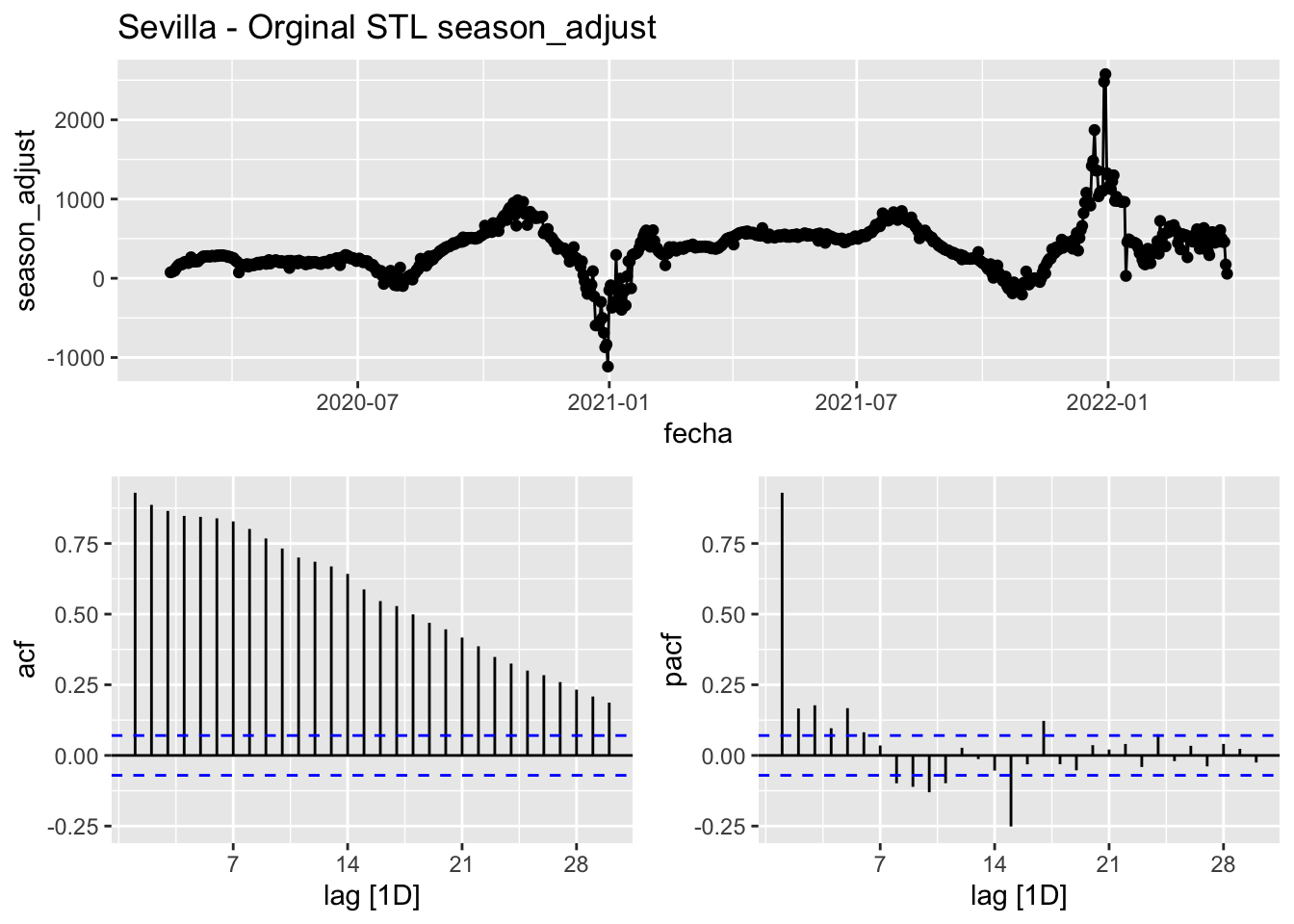
data_sevilla %>%
      model(
            STL(num_casos ~ season(window = 7) + trend(window = 7),
                robust = TRUE)
      ) %>%
      components() %>%
      gg_tsdisplay(trend, plot_type = 'partial', lag = 30) +
      labs(title="Sevilla - Orginal STL trend")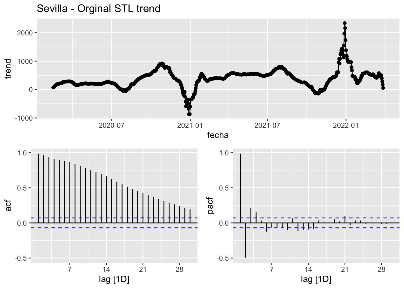
data_sevilla %>%
      model(
            STL(num_casos ~ season(window = 7) + trend(window = 7),
                robust = TRUE)
      ) %>%
      components() %>%
      gg_tsdisplay(difference(trend), plot_type = 'partial', lag = 30) +
      labs(title="Sevilla - Orginal STL trend first difference")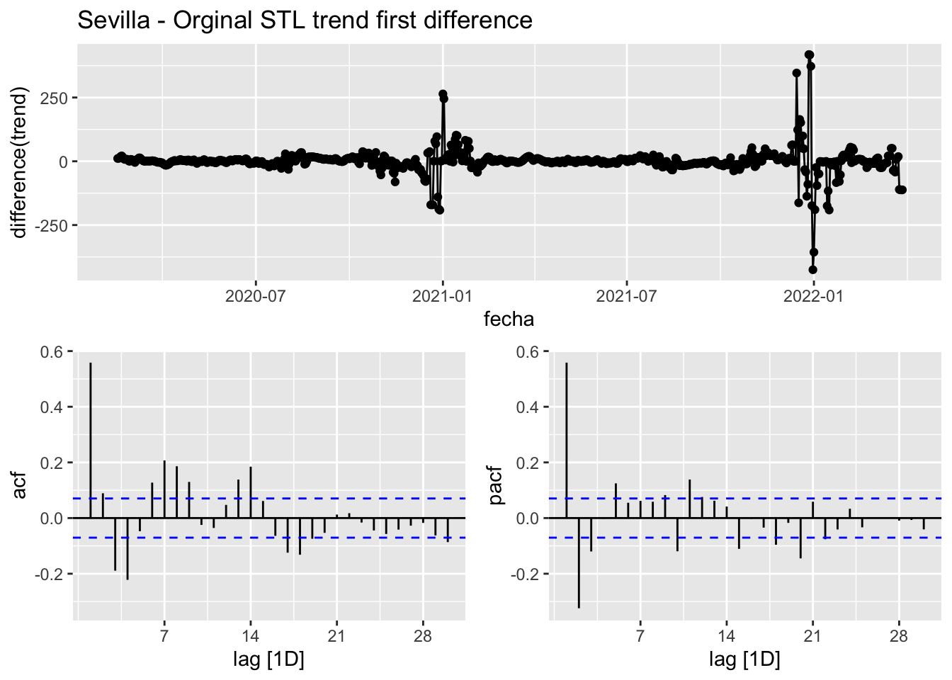
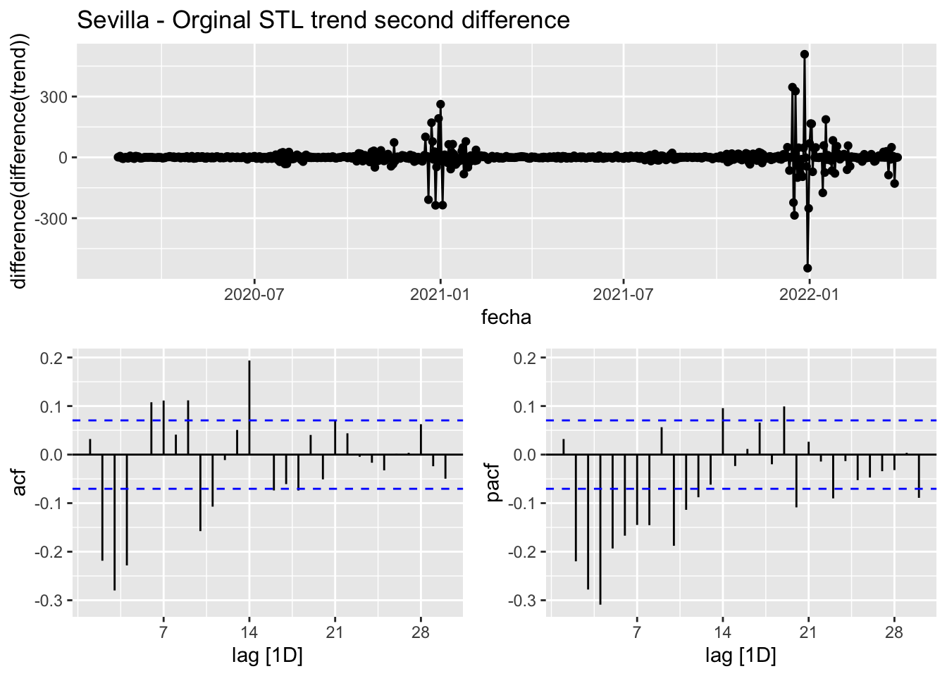
data_sevilla %>%
      model(
            STL(num_casos ~ season(window = 7) + trend(window = 7),
                robust = TRUE)
      ) %>%
      components() %>%
      gg_tsdisplay(difference(difference(trend)), plot_type = 'partial', lag = 30) +
      labs(title="Sevilla - Orginal STL trend second difference")