AEMET data

Load packages:

pacman::p_load(
      here,      # file locator
      tidyverse, # data management and ggplot2 graphics
      skimr,     # get overview of data
      janitor,   # produce and adorn tabulations and cross-tabulations
      tsibble,   # manage time series
      imputeTS,  # impute NAs for time series
      jsonlite   # read json files
)

Data is available in the Spanish State Meteorological Agency through its opendata platform link.

AEMET OpenData is a REST API (Application Programming Interface. REpresentational State Transfer) through which data can be downloaded free of charge.

AEMET OpenData allows two types of access where both allow access to the same data catalog and data download in reusable formats:

• General Access: It is a graphical access, intended for the general public. Its purpose is to allow access to data for users in a friendly way. The interaction with the data is characterized by being punctual, carried out through friendly interfaces intended for a human, directed step by step and through the choice of different options.

• AEMET OpenData API: it allows another type of interaction with the data: this interaction is characterized by the possibility of being periodic and even programmed, from any programming language, without friendly interfaces, with the possibility of self-discovery and allows information reusers to include AEMET data in their own information systems.

Last one method was used to download data from:

• Asturias airport
• Barcelona airport
• Madrid airport
• Málaga airport
• Sevilla airport

# List aemet raw json files
meteo_files <- list.files(
      path = here("data", "raw"),
      recursive = TRUE,
      full.names = TRUE,
      pattern = "*meteo.json"
)

Load and deserialize json files.

meteo_data <- map_dfr(
      .x = meteo_files, 
      .f = ~fromJSON(.x, flatten = TRUE)
) %>% as_tibble()
meteo_data

# A tibble: 4,105 × 20
   fecha    indicativo nombre provincia altitud tmed  prec  tmin  horatmin tmax 
   <chr>    <chr>      <chr>  <chr>     <chr>   <chr> <chr> <chr> <chr>    <chr>
 1 2020-01… 1212E      ASTUR… ASTURIAS  127     7,4   0,0   3,8   19:42    11,0 
 2 2020-01… 1212E      ASTUR… ASTURIAS  127     7,3   0,0   3,2   05:14    11,4 
 3 2020-01… 1212E      ASTUR… ASTURIAS  127     10,7  0,7   7,4   22:57    14,0 
 4 2020-01… 1212E      ASTUR… ASTURIAS  127     8,4   2,4   5,6   18:32    11,1 
 5 2020-01… 1212E      ASTUR… ASTURIAS  127     8,2   0,0   4,7   03:39    11,8 
 6 2020-01… 1212E      ASTUR… ASTURIAS  127     7,6   0,0   2,8   01:53    12,3 
 7 2020-01… 1212E      ASTUR… ASTURIAS  127     8,8   0,0   4,3   07:38    13,3 
 8 2020-01… 1212E      ASTUR… ASTURIAS  127     13,4  0,0   9,0   Varias   17,7 
 9 2020-01… 1212E      ASTUR… ASTURIAS  127     14,4  5,5   8,7   22:53    20,2 
10 2020-01… 1212E      ASTUR… ASTURIAS  127     8,2   0,6   4,9   23:46    11,6 
# … with 4,095 more rows, and 10 more variables: horatmax <chr>, dir <chr>,
#   velmedia <chr>, racha <chr>, horaracha <chr>, sol <chr>, presMax <chr>,
#   horaPresMax <chr>, presMin <chr>, horaPresMin <chr>

All the information corresponds to airports.

table(meteo_data$nombre)

 ASTURIAS AEROPUERTO BARCELONA AEROPUERTO    MADRID AEROPUERTO 
                 821                  821                  821 
   MÁLAGA AEROPUERTO   SEVILLA AEROPUERTO 
                 821                  821 

Data statistics:

skim(meteo_data)

Data summary

Name	meteo_data
Number of rows	4105
Number of columns	20
_______________________
Column type frequency:
character	20
________________________
Group variables	None

Variable type: character

skim_variable	n_missing	complete_rate	min	max	empty	n_unique	whitespace
fecha	0	1.00	10	10	0	821	0
indicativo	0	1.00	4	5	0	5	0
nombre	0	1.00	17	20	0	5	0
provincia	0	1.00	6	9	0	5	0
altitud	0	1.00	1	3	0	5	0
tmed	31	0.99	3	4	0	312	0
prec	6	1.00	2	4	0	243	0
tmin	31	0.99	3	5	0	315	0
horatmin	31	0.99	5	6	0	673	0
tmax	30	0.99	3	4	0	363	0
horatmax	30	0.99	5	6	0	588	0
dir	68	0.98	2	2	0	37	0
velmedia	45	0.99	3	4	0	48	0
racha	68	0.98	3	4	0	65	0
horaracha	68	0.98	5	6	0	1018	0
sol	78	0.98	3	4	0	144	0
presMax	44	0.99	5	6	0	636	0
horaPresMax	44	0.99	2	6	0	20	0
presMin	44	0.99	5	6	0	681	0
horaPresMin	44	0.99	2	6	0	26	0

Some cleaning is needed.

First of all, we will remove useless columns for further analysis and rename the others. Secondly, we will transform date to a valid format. Last but not least, we will transform numeric data to a valid numeric format.

meteo_data <- meteo_data %>% 
      select(-indicativo, -nombre, -altitud, -horatmin, -horatmax, -horaracha, -presMax, -horaPresMax, -presMin, -horaPresMin) %>% 
      mutate(
            fecha    = as.Date(fecha, format = "%Y-%m-%d"),
            tmed     = as.numeric(sub(",", ".", tmed, fixed = TRUE)),
            prec     = as.numeric(sub(",", ".", prec, fixed = TRUE)),
            tmin     = as.numeric(sub(",", ".", tmin, fixed = TRUE)),
            tmax     = as.numeric(sub(",", ".", tmax, fixed = TRUE)),
            dir      = as.numeric(sub(",", ".", dir, fixed = TRUE)),
            velmedia = as.numeric(sub(",", ".", velmedia, fixed = TRUE)),
            racha    = as.numeric(sub(",", ".", racha, fixed = TRUE)),
            sol      = as.numeric(sub(",", ".", sol, fixed = TRUE))
      ) %>% 
      rename(
            wd     = dir,
            ws     = velmedia,
            ws_max = racha
      )

Warning in mask$eval_all_mutate(quo): NAs introduced by coercion

meteo_data

# A tibble: 4,105 × 10
   fecha      provincia  tmed  prec  tmin  tmax    wd    ws ws_max   sol
   <date>     <chr>     <dbl> <dbl> <dbl> <dbl> <dbl> <dbl>  <dbl> <dbl>
 1 2020-01-01 ASTURIAS    7.4   0     3.8  11      99   2.5    7.8   7.9
 2 2020-01-02 ASTURIAS    7.3   0     3.2  11.4    22   2.8   10.3   2.8
 3 2020-01-03 ASTURIAS   10.7   0.7   7.4  14      99   2.8    9.7   1.9
 4 2020-01-04 ASTURIAS    8.4   2.4   5.6  11.1    99   3.6    7.2   0.7
 5 2020-01-05 ASTURIAS    8.2   0     4.7  11.8    13   2.5    7.2   8.6
 6 2020-01-06 ASTURIAS    7.6   0     2.8  12.3    22   3.1    8.9   6.3
 7 2020-01-07 ASTURIAS    8.8   0     4.3  13.3    99   1.9    8.9   8  
 8 2020-01-08 ASTURIAS   13.4   0     9    17.7    22   2.8    8.3   6.1
 9 2020-01-09 ASTURIAS   14.4   5.5   8.7  20.2    29   7.8   24.2   4.3
10 2020-01-10 ASTURIAS    8.2   0.6   4.9  11.6    28   2.2   16.1   1.9
# … with 4,095 more rows

In order to unify the data with other available sources, a rename of the provinces it needed.

meteo_data <- meteo_data %>% 
      mutate(
            provincia = case_when(
                  provincia == "ASTURIAS" ~ "Asturias",
                  provincia == "BARCELONA" ~ "Barcelona",
                  provincia == "MADRID" ~ "Madrid",
                  provincia == "MALAGA" ~ "Málaga",
                  provincia == "SEVILLA" ~ "Sevilla",
                  TRUE ~ provincia
            )
      )
unique(meteo_data$provincia)

[1] "Asturias"  "Barcelona" "Madrid"    "Málaga"    "Sevilla"  

The data has missing information.

skim(meteo_data)

Data summary

Name	meteo_data
Number of rows	4105
Number of columns	10
_______________________
Column type frequency:
character	1
Date	1
numeric	8
________________________
Group variables	None

Variable type: character

skim_variable	n_missing	complete_rate	min	max	empty	n_unique	whitespace
provincia	0	1	6	9	0	5	0

Variable type: Date

skim_variable	n_missing	complete_rate	min	max	median	n_unique
fecha	0	1	2020-01-01	2022-03-31	2021-02-14	821

Variable type: numeric

skim_variable	n_missing	complete_rate	mean	sd	p0	p25	p50	p75	p100	hist
tmed	31	0.99	16.60	6.44	-6.2	12.0	15.6	21.0	34.5	▁▂▇▅▂
prec	149	0.96	1.74	6.20	0.0	0.0	0.0	0.1	87.9	▇▁▁▁▁
tmin	31	0.99	11.66	6.22	-13.4	7.4	11.3	16.0	27.5	▁▁▇▇▂
tmax	30	0.99	21.53	7.28	0.3	16.2	20.3	26.4	44.9	▁▇▇▃▁
wd	68	0.98	41.65	36.42	1.0	15.0	26.0	99.0	99.0	▆▇▁▁▆
ws	45	0.99	3.71	1.74	0.3	2.5	3.3	4.4	18.9	▇▅▁▁▁
ws_max	68	0.98	10.22	3.62	2.5	7.8	9.7	11.7	31.9	▆▇▂▁▁
sol	78	0.98	6.94	4.13	0.0	3.4	7.7	10.2	14.3	▇▅▆▇▅

An interpolation for each provinces will be carried out in order to have the maximum information available.

Asturias

meteo_asturias <- meteo_data %>% 
      filter(provincia == "Asturias")

# NA imputation test
imp <- na_interpolation(meteo_asturias)

NAs imputed to average temperature:

ggplot_na_imputations(meteo_asturias$tmed, imp$tmed)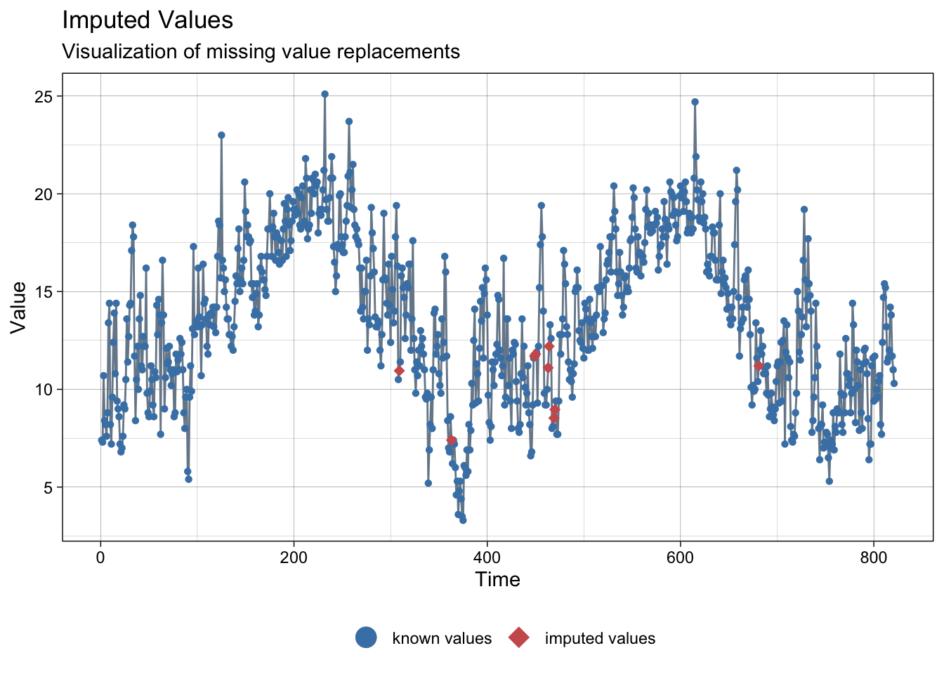

NAs imputed to precipitations:

ggplot_na_imputations(meteo_asturias$prec, imp$prec)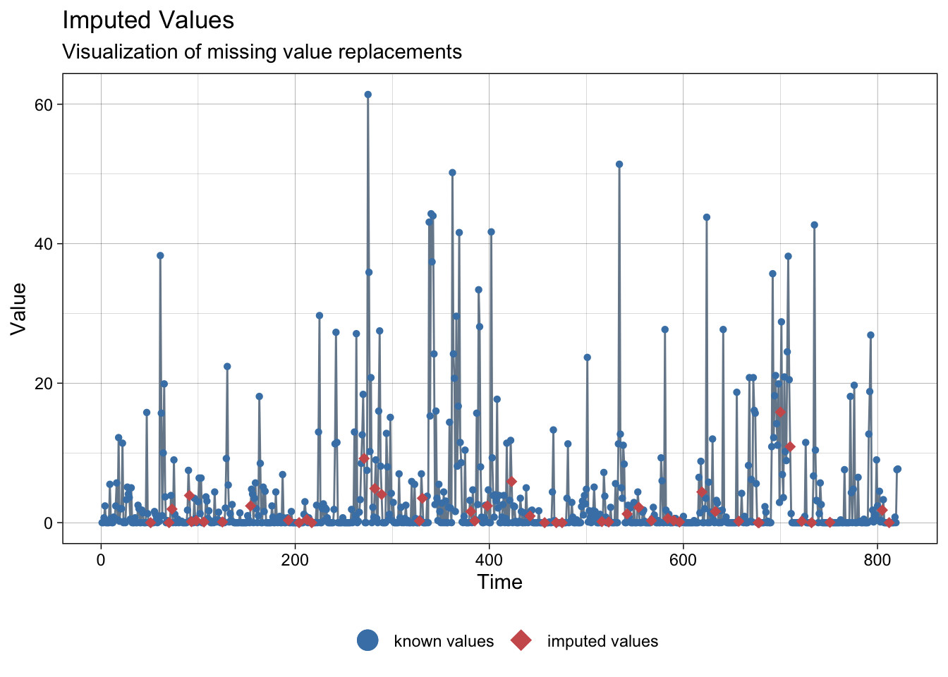

NAs imputed to wind speed:

ggplot_na_imputations(meteo_asturias$ws, imp$ws)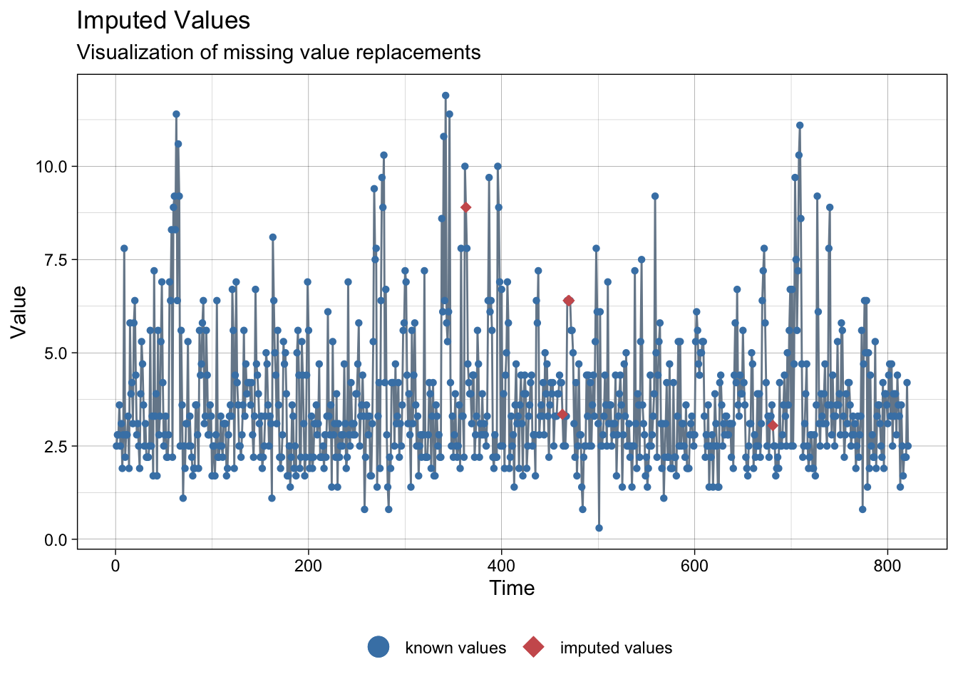

Data interpolation test looks good, so we proceed to charge it:

meteo_asturias <- na_interpolation(meteo_asturias)

Barcelona

meteo_barcelona <- meteo_data %>% 
      filter(provincia == "Barcelona")

# NA imputation test
imp <- na_interpolation(meteo_barcelona)

NAs imputed to average temperature:

ggplot_na_imputations(meteo_barcelona$tmed, imp$tmed)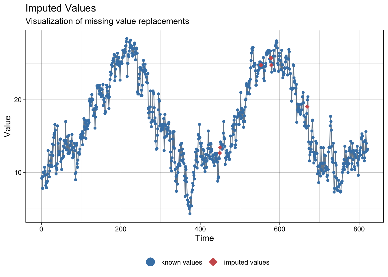

NAs imputed to precipitations:

ggplot_na_imputations(meteo_barcelona$prec, imp$prec)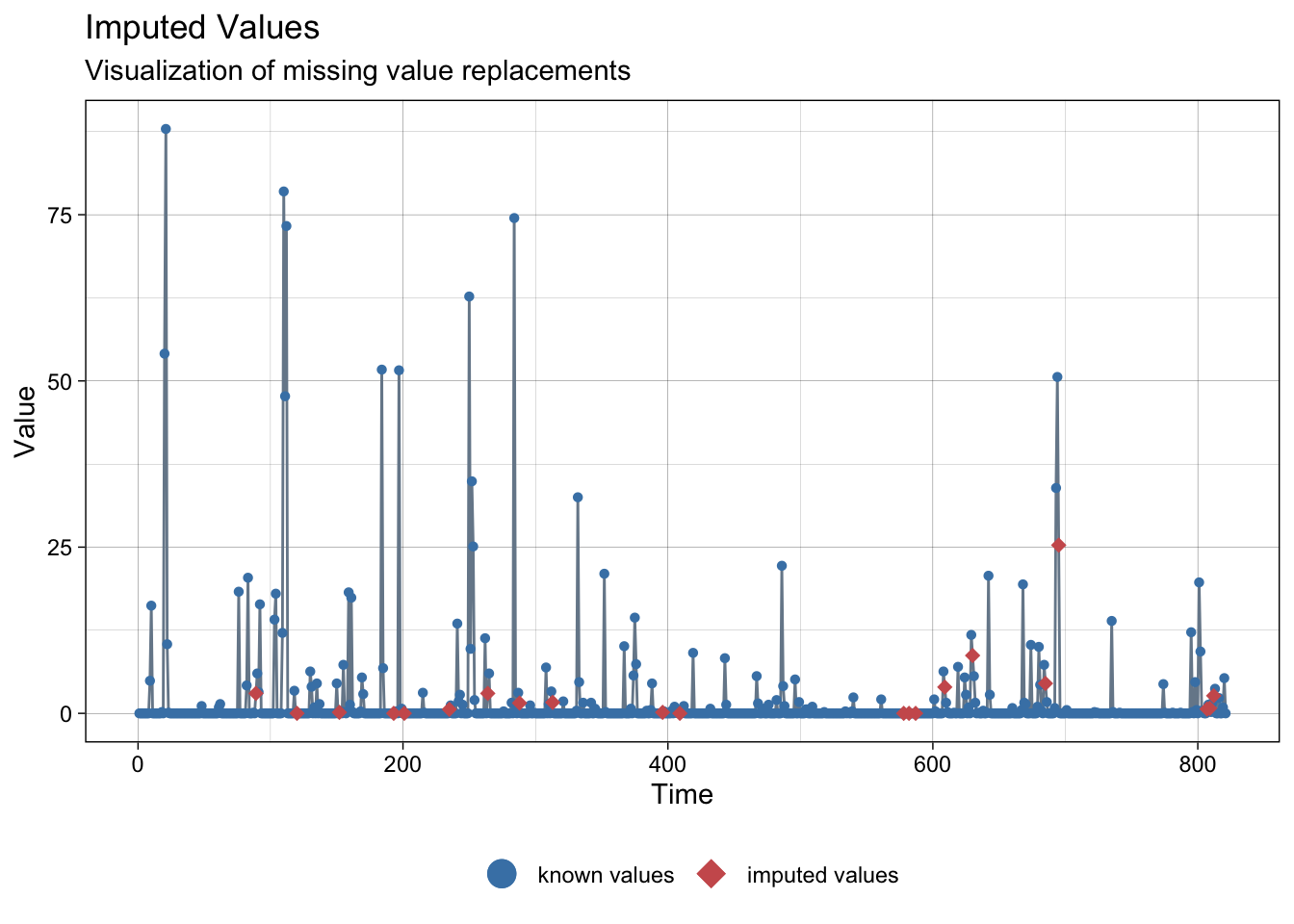

NAs imputed to wind speed:

ggplot_na_imputations(meteo_barcelona$ws, imp$ws)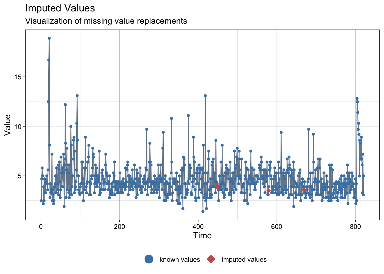

Data interpolation test looks good, so we proceed to charge it:

meteo_barcelona <- na_interpolation(meteo_barcelona)

Madrid

meteo_madrid <- meteo_data %>% 
      filter(provincia == "Madrid")

# NA imputation test
imp <- na_interpolation(meteo_madrid)

NAs imputed to average temperature:

print("There are not NAs!")

[1] "There are not NAs!"

NAs imputed to precipitations:

ggplot_na_imputations(meteo_madrid$prec, imp$prec)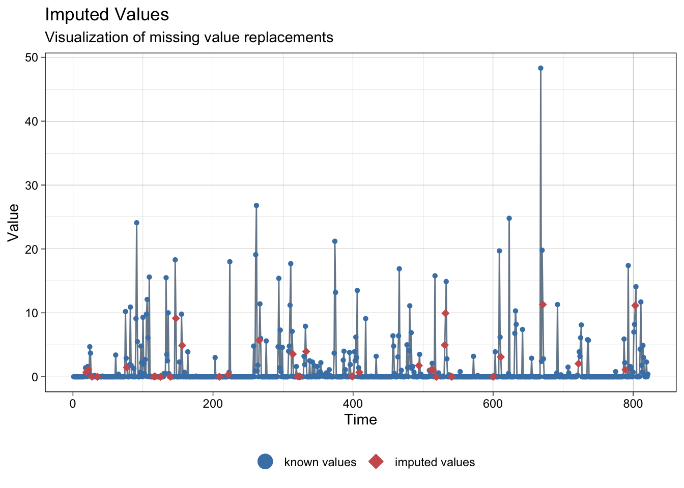

NAs imputed to wind speed:

ggplot_na_imputations(meteo_madrid$ws, imp$ws)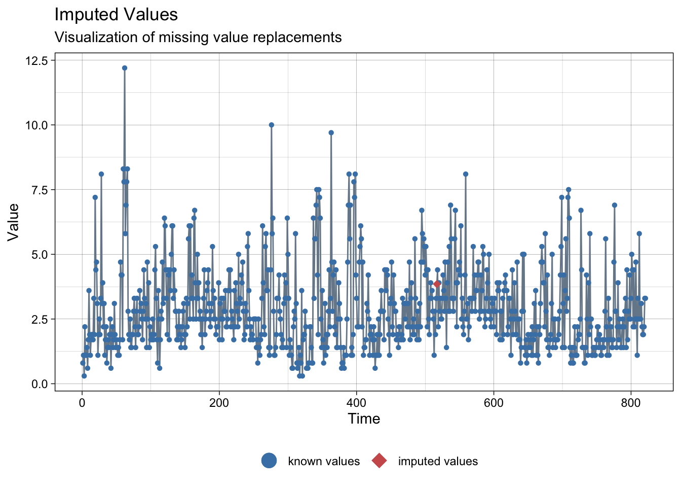

Data interpolation test looks good, so we proceed to charge it:

meteo_madrid <- na_interpolation(meteo_madrid)

Malaga

meteo_malaga <- meteo_data %>% 
      filter(provincia == "Málaga")

# NA imputation test
imp <- na_interpolation(meteo_malaga)

NAs imputed to average temperature:

ggplot_na_imputations(meteo_malaga$tmed, imp$tmed)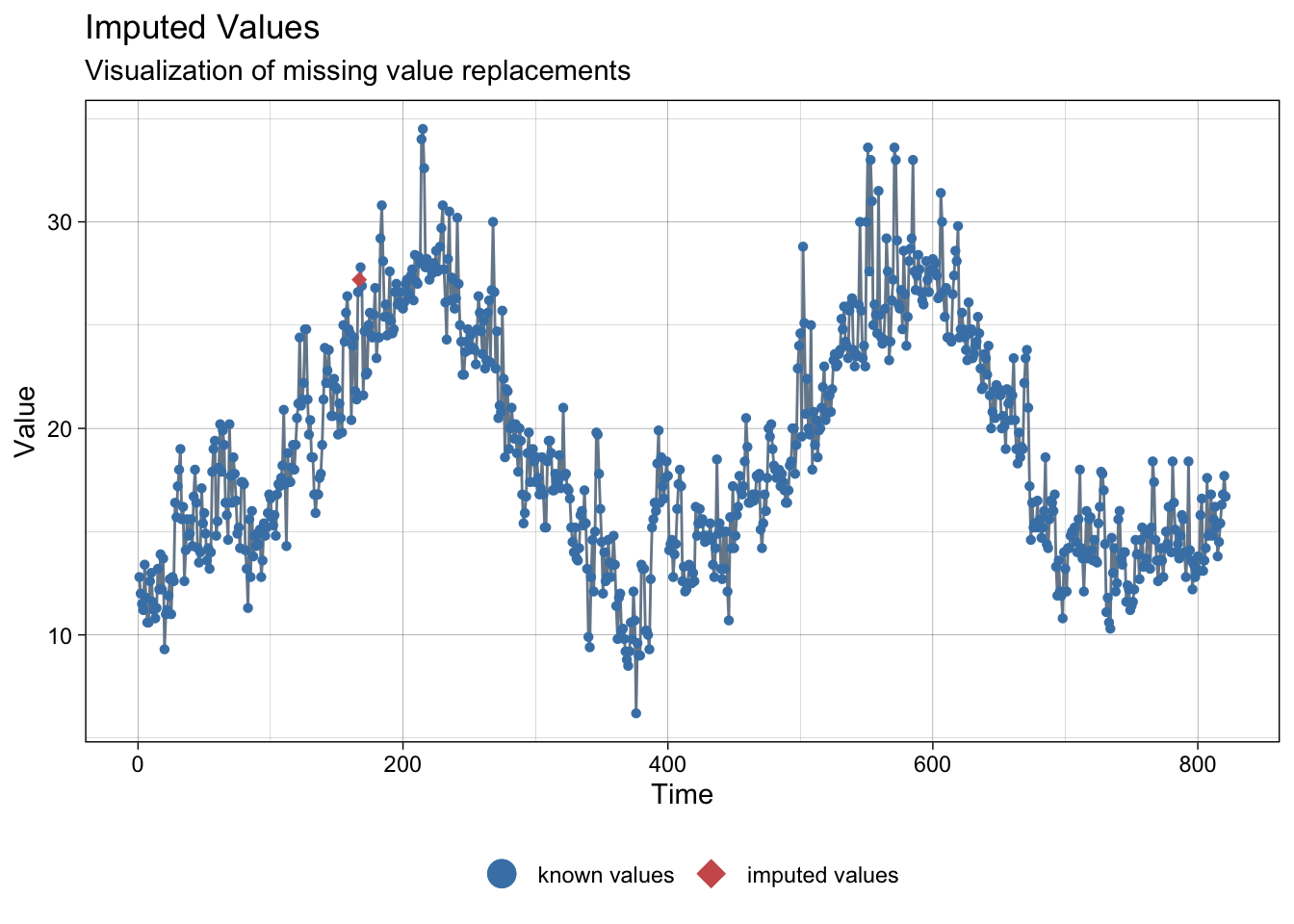

NAs imputed to precipitations:

ggplot_na_imputations(meteo_malaga$prec, imp$prec)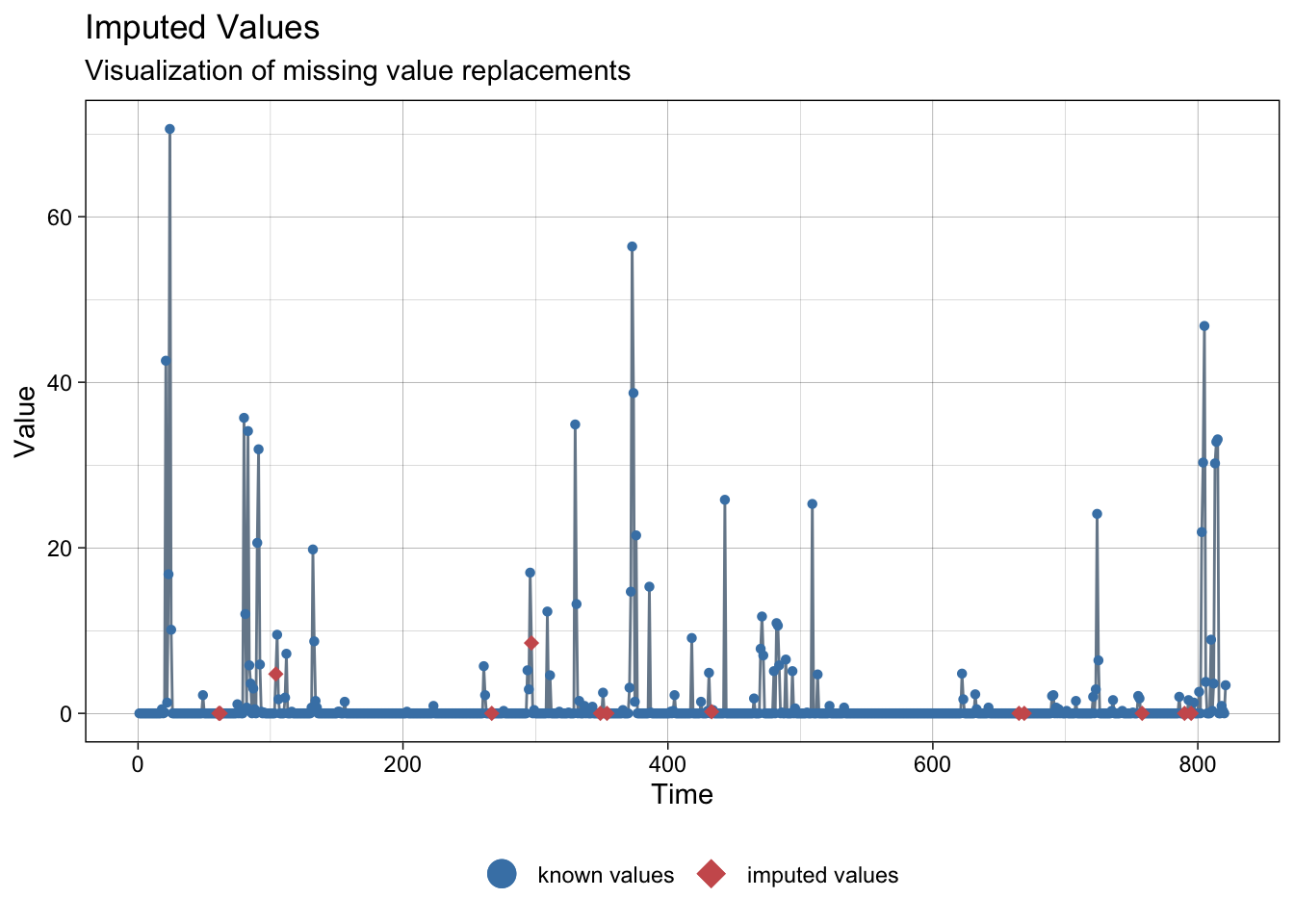

NAs imputed to wind speed:

print("There are not NAs!")

[1] "There are not NAs!"

Data interpolation test looks good, so we proceed to charge it:

meteo_malaga <- na_interpolation(meteo_malaga)

Sevilla

meteo_sevilla <- meteo_data %>% 
      filter(provincia == "Sevilla")

# NA imputation test
imp <- na_interpolation(meteo_sevilla)

NAs imputed to average temperature:

ggplot_na_imputations(meteo_sevilla$tmed, imp$tmed)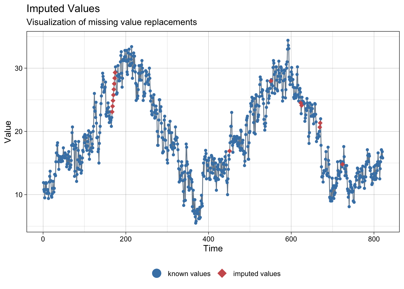

NAs imputed to precipitations:

ggplot_na_imputations(meteo_sevilla$prec, imp$prec)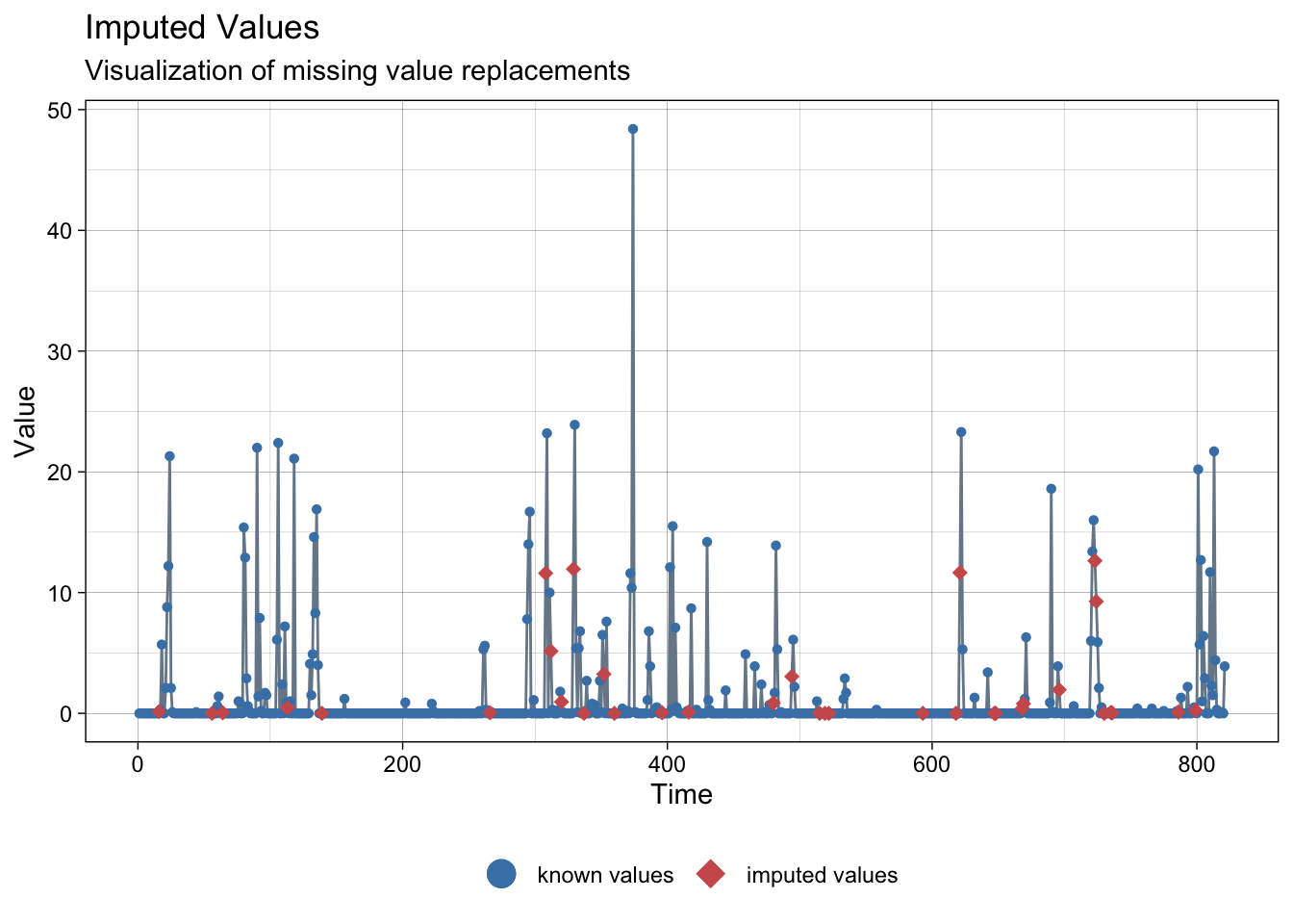

NAs imputed to wind speed:

ggplot_na_imputations(meteo_sevilla$ws, imp$ws)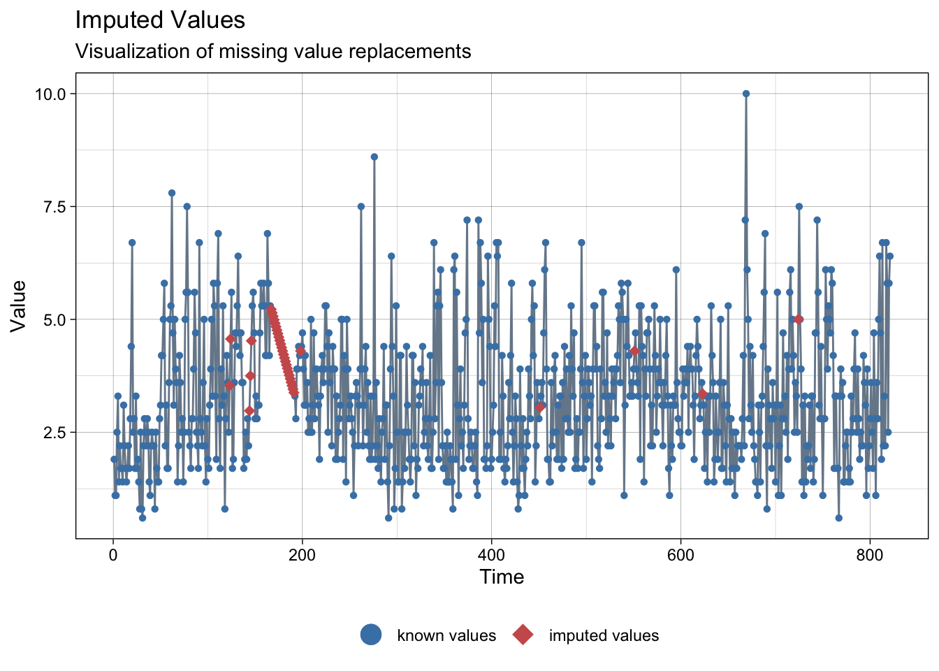

Data interpolation test looks good, so we proceed to charge it:

meteo_sevilla <- na_interpolation(meteo_sevilla)

Data combination

meteo_data_completed <- meteo_asturias %>% 
      rbind(meteo_barcelona) %>% 
      rbind(meteo_madrid) %>% 
      rbind(meteo_malaga) %>% 
      rbind(meteo_sevilla)
unique(meteo_data_completed$provincia)

[1] "Asturias"  "Barcelona" "Madrid"    "Málaga"    "Sevilla"  

Final statistics:

skim(meteo_data_completed)

Data summary

Name	meteo_data_completed
Number of rows	4105
Number of columns	10
_______________________
Column type frequency:
character	1
Date	1
numeric	8
________________________
Group variables	None

Variable type: character

skim_variable	n_missing	complete_rate	min	max	empty	n_unique	whitespace
provincia	0	1	6	9	0	5	0

Variable type: Date

skim_variable	n_missing	complete_rate	min	max	median	n_unique
fecha	0	1	2020-01-01	2022-03-31	2021-02-14	821

Variable type: numeric

skim_variable	n_missing	complete_rate	mean	sd	p0	p25	p50	p75	p100	hist
tmed	0	1	16.62	6.45	-6.2	12.0	15.6	21.10	34.5	▁▂▇▅▂
prec	0	1	1.76	6.13	0.0	0.0	0.0	0.20	87.9	▇▁▁▁▁
tmin	0	1	11.68	6.22	-13.4	7.4	11.3	16.10	27.5	▁▁▇▇▂
tmax	0	1	21.56	7.30	0.3	16.2	20.3	26.40	44.9	▁▇▇▃▁
wd	0	1	41.79	36.26	1.0	15.0	26.0	99.00	99.0	▆▇▁▁▆
ws	0	1	3.72	1.73	0.3	2.5	3.6	4.40	18.9	▇▅▁▁▁
ws_max	0	1	10.24	3.61	2.5	7.8	9.7	12.15	31.9	▅▇▂▁▁
sol	0	1	6.97	4.12	0.0	3.5	7.7	10.30	14.3	▇▅▆▇▅

The final data looks like:

meteo_data_completed

# A tibble: 4,105 × 10
   fecha      provincia  tmed  prec  tmin  tmax    wd    ws ws_max   sol
   <date>     <chr>     <dbl> <dbl> <dbl> <dbl> <dbl> <dbl>  <dbl> <dbl>
 1 2020-01-01 Asturias    7.4   0     3.8  11      99   2.5    7.8   7.9
 2 2020-01-02 Asturias    7.3   0     3.2  11.4    22   2.8   10.3   2.8
 3 2020-01-03 Asturias   10.7   0.7   7.4  14      99   2.8    9.7   1.9
 4 2020-01-04 Asturias    8.4   2.4   5.6  11.1    99   3.6    7.2   0.7
 5 2020-01-05 Asturias    8.2   0     4.7  11.8    13   2.5    7.2   8.6
 6 2020-01-06 Asturias    7.6   0     2.8  12.3    22   3.1    8.9   6.3
 7 2020-01-07 Asturias    8.8   0     4.3  13.3    99   1.9    8.9   8  
 8 2020-01-08 Asturias   13.4   0     9    17.7    22   2.8    8.3   6.1
 9 2020-01-09 Asturias   14.4   5.5   8.7  20.2    29   7.8   24.2   4.3
10 2020-01-10 Asturias    8.2   0.6   4.9  11.6    28   2.2   16.1   1.9
# … with 4,095 more rows