pacman::p_load(
      here,      # file locator
      tidyverse, # data management and ggplot2 graphics
      skimr,     # get overview of data
      janitor,   # produce and adorn tabulations and cross-tabulations
      tsibble,
      fable,
      feasts,
      fabletools,
      lubridate
)

covid_data <- readRDS(here("data", "clean", "final_covid_data.rds"))Multivariate (temperature) prediction
Load packages:
The temporal limits of our prediction will be:
- Data as of June 14th 2020 which is considered the beginning of the second epidemiological period in Spain
- In the first case scenario, data previous the start of the sixth wave of covid-19 (14 oct 2021).
- In the second case scenario, all the available data (limited by mobility information 29 dec 2021)
Before sixth epidemiological period
Asturias
data_asturias <- covid_data %>%
      filter(provincia == "Asturias") %>%
      filter(fecha > as.Date("2020-06-14", format = "%Y-%m-%d")) %>%
      select(provincia, fecha, num_casos, tmed) %>%
      drop_na() %>%
      as_tsibble(key = provincia, index = fecha)
data_asturias
# A tsibble: 653 x 4 [1D]
# Key: provincia [1]
provincia fecha num_casos tmed
<chr> <date> <dbl> <dbl>
1 Asturias 2020-06-15 0 16
2 Asturias 2020-06-16 1 15.6
3 Asturias 2020-06-17 0 15.6
4 Asturias 2020-06-18 0 15.1
5 Asturias 2020-06-19 0 14.8
6 Asturias 2020-06-20 0 16.8
7 Asturias 2020-06-21 0 18.2
8 Asturias 2020-06-22 0 18.2
9 Asturias 2020-06-23 0 20
10 Asturias 2020-06-24 0 18.2
# … with 643 more rowsdata_asturias_train <- data_asturias %>%
filter(fecha <= as.Date("2021-10-14", format = "%Y-%m-%d"))
summary(data_asturias_train$fecha) Min. 1st Qu. Median Mean 3rd Qu. Max.
"2020-06-15" "2020-10-14" "2021-02-13" "2021-02-13" "2021-06-14" "2021-10-14" data_asturias_test <- data_asturias %>%
filter(fecha > as.Date("2021-10-14", format = "%Y-%m-%d"))
summary(data_asturias_test$fecha) Min. 1st Qu. Median Mean 3rd Qu. Max.
"2021-10-15" "2021-11-25" "2022-01-05" "2022-01-05" "2022-02-15" "2022-03-29" # Lamba for num_casos
lambda_asturias_casos <- data_asturias %>%
features(num_casos, features = guerrero) %>%
pull(lambda_guerrero)
lambda_asturias_casos[1] 0.2278229# Lamba for average temp
lambda_asturias_tmed <- data_asturias %>%
features(tmed, features = guerrero) %>%
pull(lambda_guerrero)
lambda_asturias_tmed[1] 1.056074fit_model <- data_asturias_train %>%
model(
arima_at1 = ARIMA(box_cox(num_casos, lambda_asturias_casos) ~
box_cox(tmed, lambda_asturias_tmed)),
arima_at2 = ARIMA(box_cox(num_casos, lambda_asturias_casos) ~
box_cox(tmed, lambda_asturias_tmed),
stepwise = FALSE, approx = FALSE),
Snaive = SNAIVE(box_cox(num_casos, lambda_asturias_casos))
)
# Show and report model
fit_model# A mable: 1 x 4
# Key: provincia [1]
provincia arima_at1 arima_at2
<chr> <model> <model>
1 Asturias <LM w/ ARIMA(3,1,1)(2,0,0)[7] errors> <LM w/ ARIMA(2,1,4) errors>
# … with 1 more variable: Snaive <model>glance(fit_model)# A tibble: 3 × 9
provincia .model sigma2 log_lik AIC AICc BIC ar_roots ma_roots
<chr> <chr> <dbl> <dbl> <dbl> <dbl> <dbl> <list> <list>
1 Asturias arima_at1 0.946 -673. 1362. 1362. 1396. <cpl [17]> <cpl [1]>
2 Asturias arima_at2 0.912 -664. 1345. 1345. 1378. <cpl [2]> <cpl [4]>
3 Asturias Snaive 2.32 NA NA NA NA <NULL> <NULL> fit_model %>%
pivot_longer(-provincia,
names_to = ".model",
values_to = "orders") %>%
left_join(glance(fit_model), by = c("provincia", ".model")) %>%
arrange(AICc) %>%
select(.model:BIC)# A mable: 3 x 7
# Key: .model [3]
.model orders sigma2 log_lik AIC AICc BIC
<chr> <model> <dbl> <dbl> <dbl> <dbl> <dbl>
1 arima_… <LM w/ ARIMA(2,1,4) errors> 0.912 -664. 1345. 1345. 1378.
2 arima_… <LM w/ ARIMA(3,1,1)(2,0,0)[7] errors> 0.946 -673. 1362. 1362. 1396.
3 Snaive <SNAIVE> 2.32 NA NA NA NA # We use a Ljung-Box test >> large p-value, confirms residuals are similar / considered to white noise
fit_model %>%
select(Snaive) %>%
gg_tsresiduals()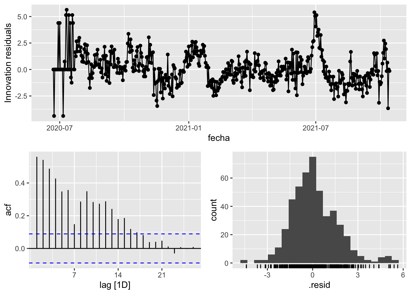
fit_model %>%
      select(arima_at1) %>%
      gg_tsresiduals()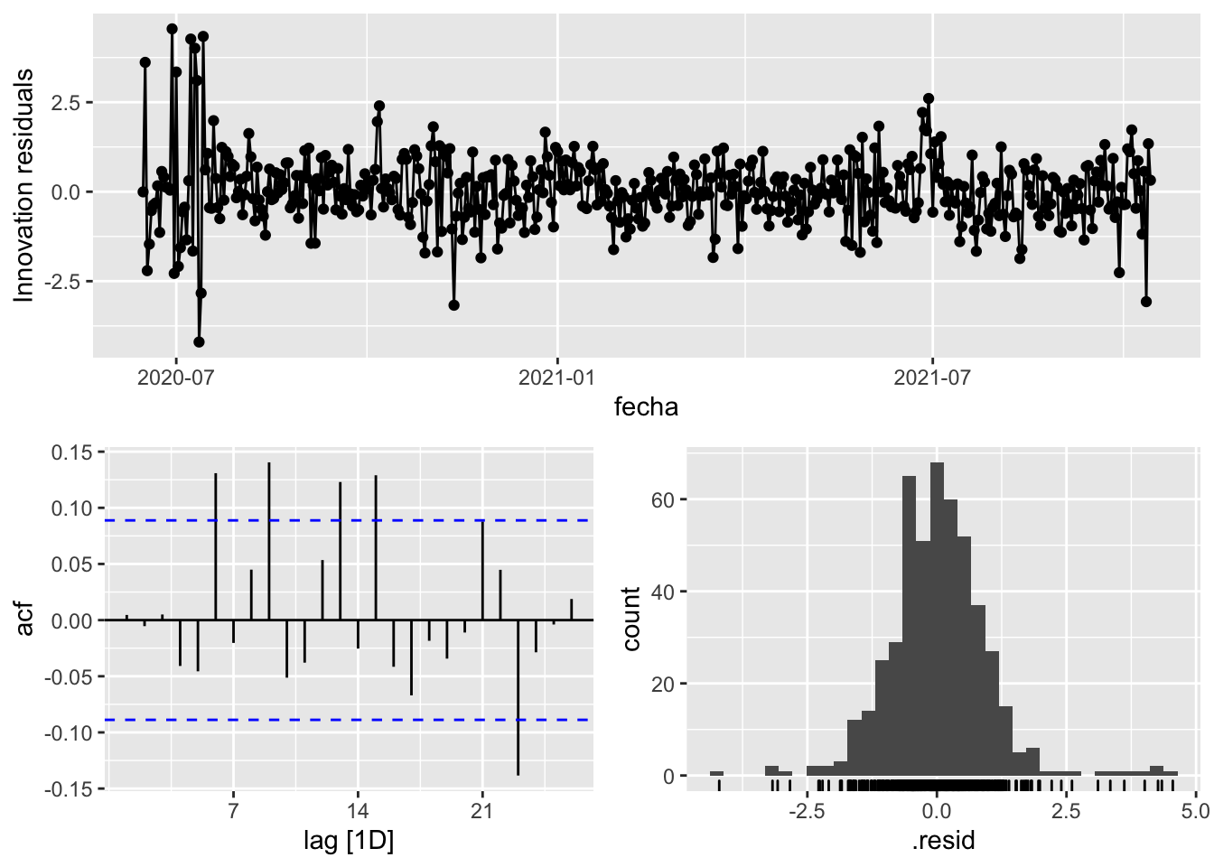
fit_model %>%
      select(arima_at2) %>%
      gg_tsresiduals()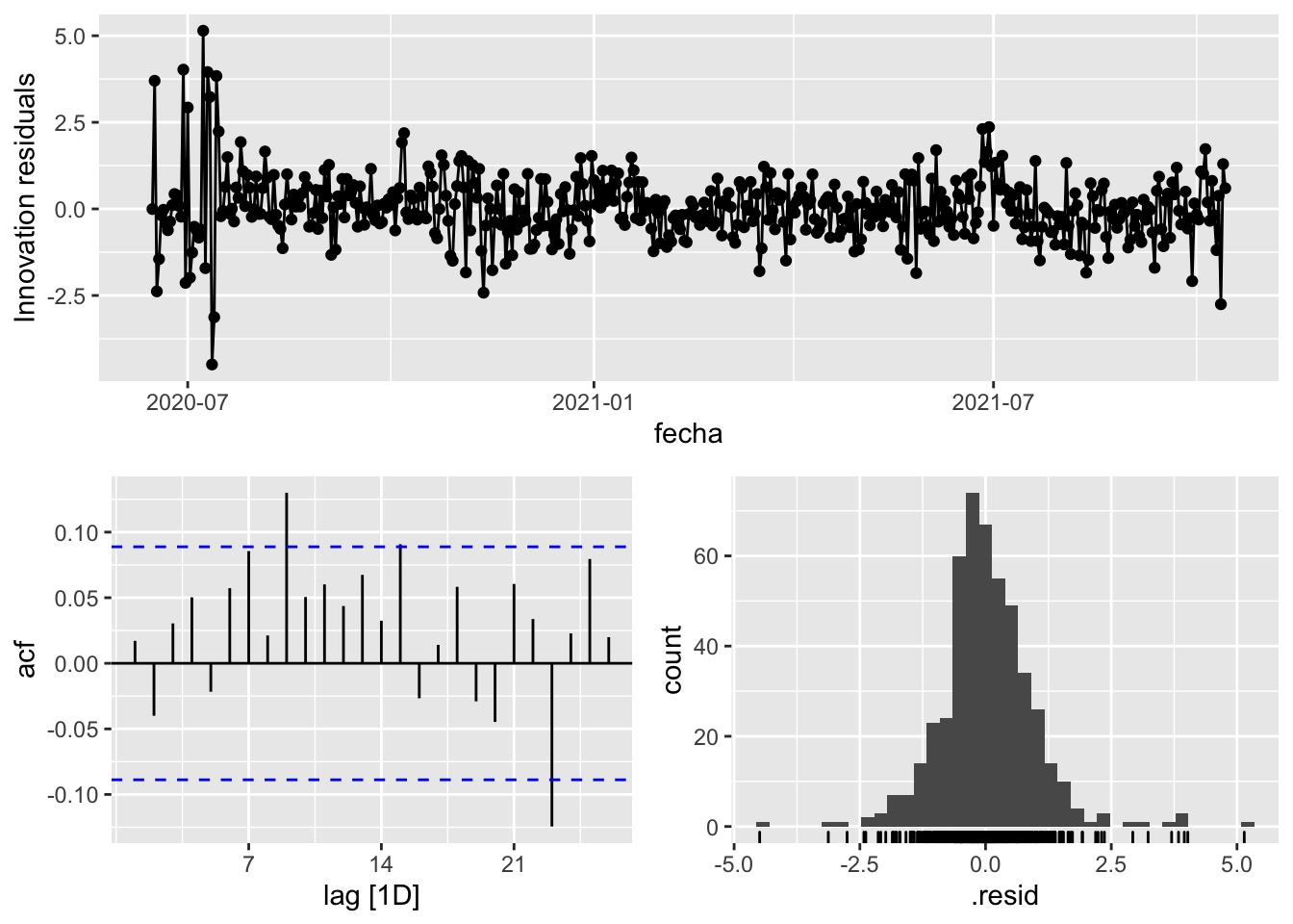
augment(fit_model) %>%
      features(.innov, ljung_box, lag=7)
# A tibble: 3 × 4
provincia .model lb_stat lb_pvalue
<chr> <chr> <dbl> <dbl>
1 Asturias arima_at1 10.6 0.159
2 Asturias arima_at2 8.12 0.322
3 Asturias Snaive 629. 0 augment(fit_model) %>%
features(.innov, ljung_box, lag=14)# A tibble: 3 × 4
provincia .model lb_stat lb_pvalue
<chr> <chr> <dbl> <dbl>
1 Asturias arima_at1 32.8 0.00309
2 Asturias arima_at2 23.6 0.0509
3 Asturias Snaive 892. 0 augment(fit_model) %>%
features(.innov, ljung_box, lag=21)# A tibble: 3 × 4
provincia .model lb_stat lb_pvalue
<chr> <chr> <dbl> <dbl>
1 Asturias arima_at1 49.1 0.000485
2 Asturias arima_at2 33.3 0.0432
3 Asturias Snaive 927. 0 augment(fit_model) %>%
features(.innov, ljung_box, lag=90)# A tibble: 3 × 4
provincia .model lb_stat lb_pvalue
<chr> <chr> <dbl> <dbl>
1 Asturias arima_at1 118. 0.0237
2 Asturias arima_at2 86.6 0.582
3 Asturias Snaive 1195. 0 # To predict future values of infections, we need to pass the model future/prediction values of the complementary variables tmed and mobility
# We are going to select those from the test dataset
data_fc_h7 <- data_asturias_test %>%
select(-num_casos) %>%
slice(1:7)
data_fc_h14 <- data_asturias_test %>%
select(-num_casos) %>%
slice(1:14)
data_fc_h21 <- data_asturias_test %>%
select(-num_casos) %>%
slice(1:21)
data_fc_h90 <- data_asturias_test %>%
select(-num_casos) %>%
slice(1:90)# Significant spikes out of 30 is still consistent with white noise
# To be sure, use a Ljung-Box test, which has a large p-value, confirming that
# the residuals are similar to white noise.
# Note that the alternative models also passed this test.
#
# Forecast
fc_h7 <- fabletools::forecast(fit_model, new_data = data_fc_h7)
fc_h14 <- fabletools::forecast(fit_model, new_data = data_fc_h14)
fc_h21 <- fabletools::forecast(fit_model, new_data = data_fc_h21)
fc_h90 <- fabletools::forecast(fit_model, new_data = data_fc_h90)7 days
# Plots
fc_h7 %>%
      autoplot(
            data_asturias_test %>%
                  filter(fecha <= as.Date("2021-10-14", format = "%Y-%m-%d")+days(9))
      ) +
      labs(y = "Nº cases", title = "Asturias - forecast h7")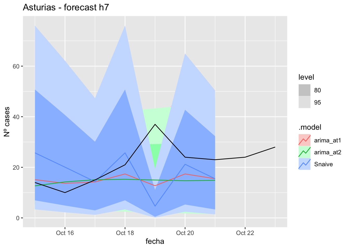
fc_h7 %>%
      autoplot(
            data_asturias %>%
                  filter(fecha <= as.Date("2021-10-14", format = "%Y-%m-%d")+days(9) &
                               fecha > as.Date("2021-07-01", format = "%Y-%m-%d"))
      ) +
      labs(y = "Nº cases", title = "Asturias - forecast h7")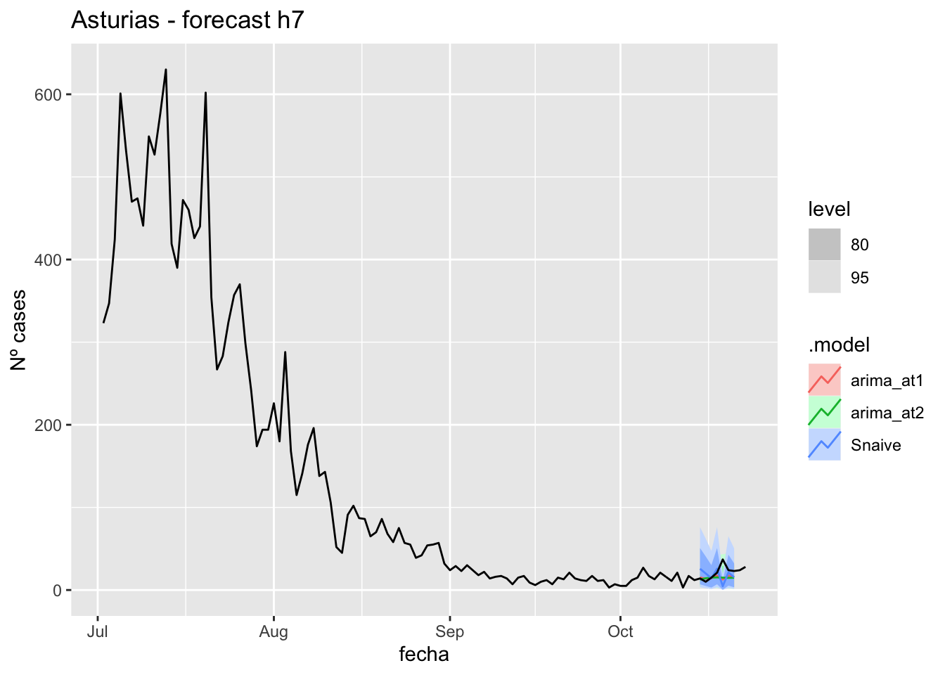
# Accuracy
fabletools::accuracy(fc_h7, data_asturias)
# A tibble: 3 × 11
.model provincia .type ME RMSE MAE MPE MAPE MASE RMSSE ACF1
<chr> <chr> <chr> <dbl> <dbl> <dbl> <dbl> <dbl> <dbl> <dbl> <dbl>
1 arima_at1 Asturias Test 5.43 10.1 6.80 14.8 27.6 0.137 0.123 0.198
2 arima_at2 Asturias Test 6.02 9.93 7.26 18.2 30.5 0.146 0.121 0.384
3 Snaive Asturias Test 2.41 14.0 9.98 -10.1 49.0 0.201 0.171 0.0076614 days
# Plots
fc_h14 %>%
      autoplot(
            data_asturias_test %>%
                  filter(fecha <= as.Date("2021-10-14", format = "%Y-%m-%d")+days(16))
      ) +
      labs(y = "Nº cases", title = "Asturias - forecast h14")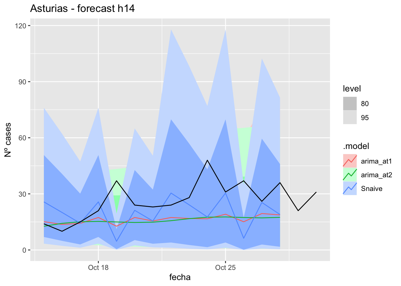
fc_h14 %>%
      autoplot(
            data_asturias %>%
                  filter(fecha <= as.Date("2021-10-14", format = "%Y-%m-%d")+days(16) &
                               fecha > as.Date("2021-07-01", format = "%Y-%m-%d"))
      ) +
      labs(y = "Nº cases", title = "Asturias - forecast h14")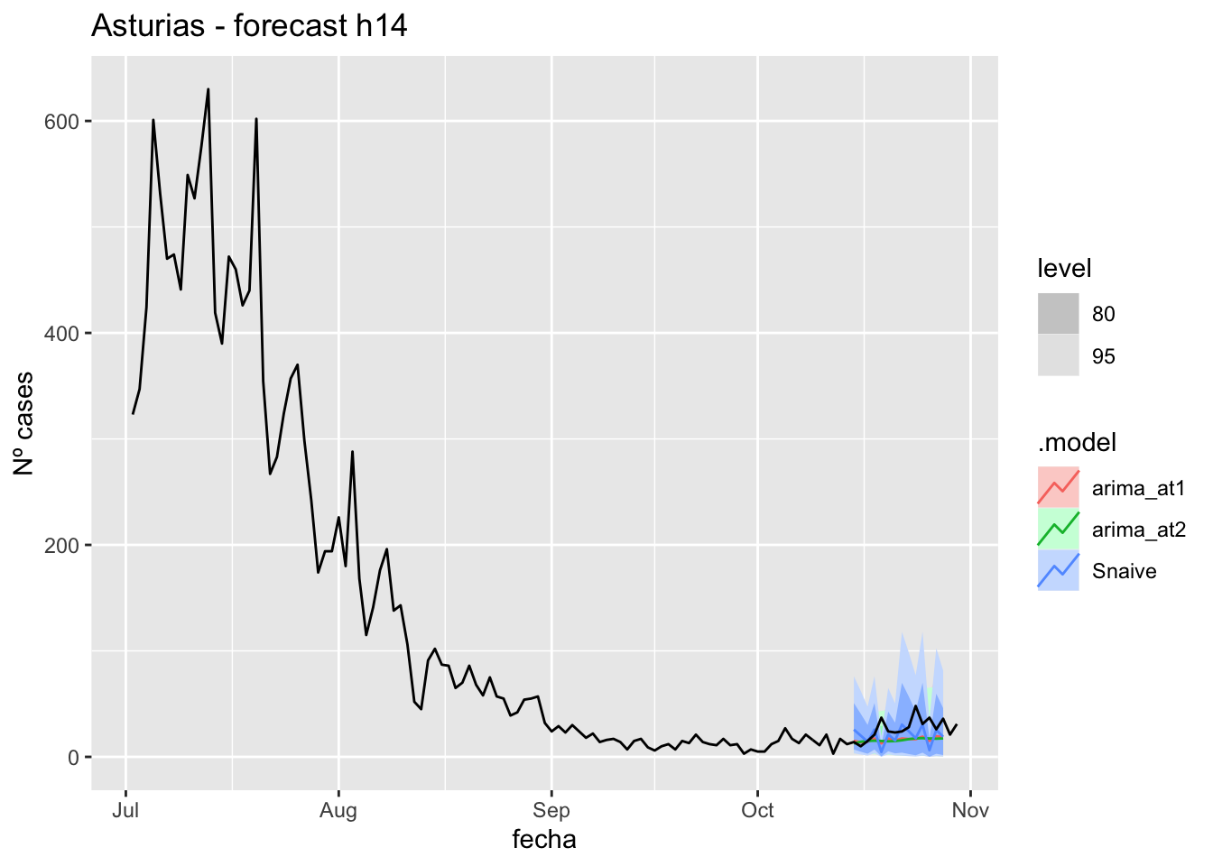
# Accuracy
fabletools::accuracy(fc_h14, data_asturias)
# A tibble: 3 × 11
.model provincia .type ME RMSE MAE MPE MAPE MASE RMSSE ACF1
<chr> <chr> <chr> <dbl> <dbl> <dbl> <dbl> <dbl> <dbl> <dbl> <dbl>
1 arima_at1 Asturias Test 10.3 14.2 11.0 29.1 35.5 0.222 0.173 0.171
2 arima_at2 Asturias Test 10.9 14.1 11.5 32.0 38.1 0.232 0.172 0.303
3 Snaive Asturias Test 6.69 16.0 11.4 8.17 41.5 0.229 0.195 -0.15621 days
# Plots
fc_h21 %>%
      autoplot(
            data_asturias_test %>%
                  filter(fecha <= as.Date("2021-10-14", format = "%Y-%m-%d")+days(23))
      ) +
      labs(y = "Nº cases", title = "Asturias - forecast h21")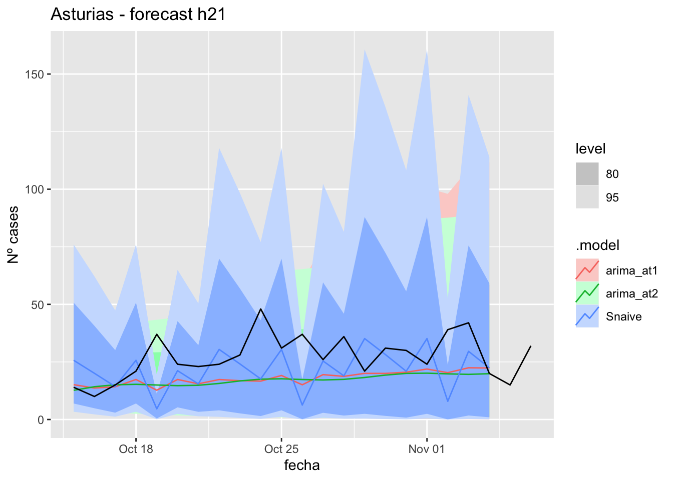
fc_h21 %>%
      autoplot(
            data_asturias %>%
                  filter(fecha <= as.Date("2021-10-14", format = "%Y-%m-%d")+days(23) &
                               fecha > as.Date("2021-07-01", format = "%Y-%m-%d"))
      ) +
      labs(y = "Nº cases", title = "Asturias - forecast h21")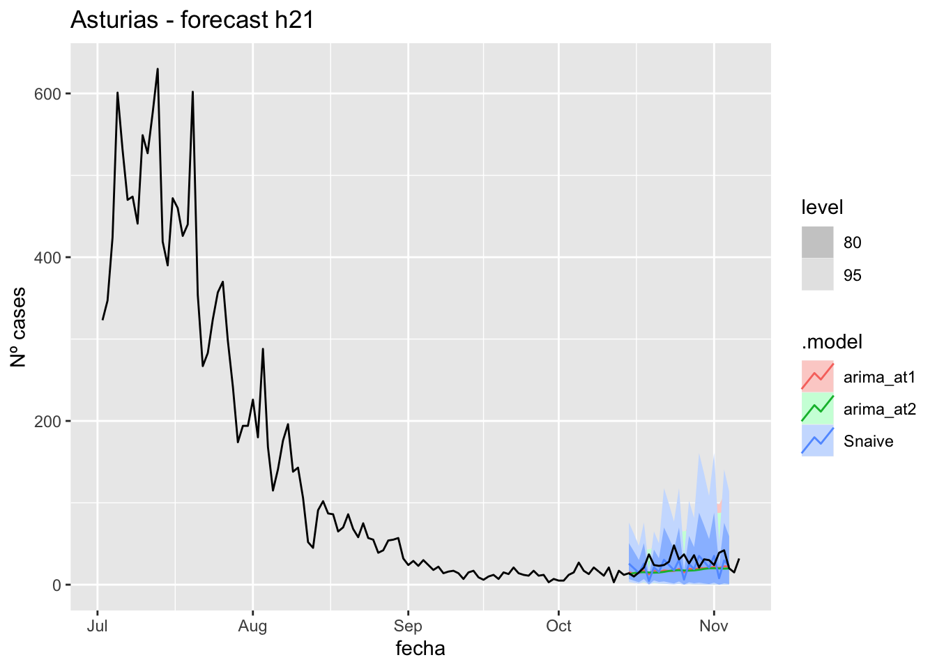
# Accuracy
fabletools::accuracy(fc_h21, data_asturias)
# A tibble: 3 × 11
.model provincia .type ME RMSE MAE MPE MAPE MASE RMSSE ACF1
<chr> <chr> <chr> <dbl> <dbl> <dbl> <dbl> <dbl> <dbl> <dbl> <dbl>
1 arima_at1 Asturias Test 9.72 13.4 10.4 27.1 32.5 0.209 0.164 0.0341
2 arima_at2 Asturias Test 10.6 13.7 11.0 31.0 35.1 0.222 0.167 0.127
3 Snaive Asturias Test 5.77 15.6 11.5 6.52 40.8 0.232 0.190 -0.223 90 days
# Plots
fc_h90 %>%
      autoplot(
            data_asturias_test %>%
                  filter(fecha <= as.Date("2021-10-14", format = "%Y-%m-%d")+days(92))
      ) +
      labs(y = "Nº cases", title = "Asturias - forecast h90")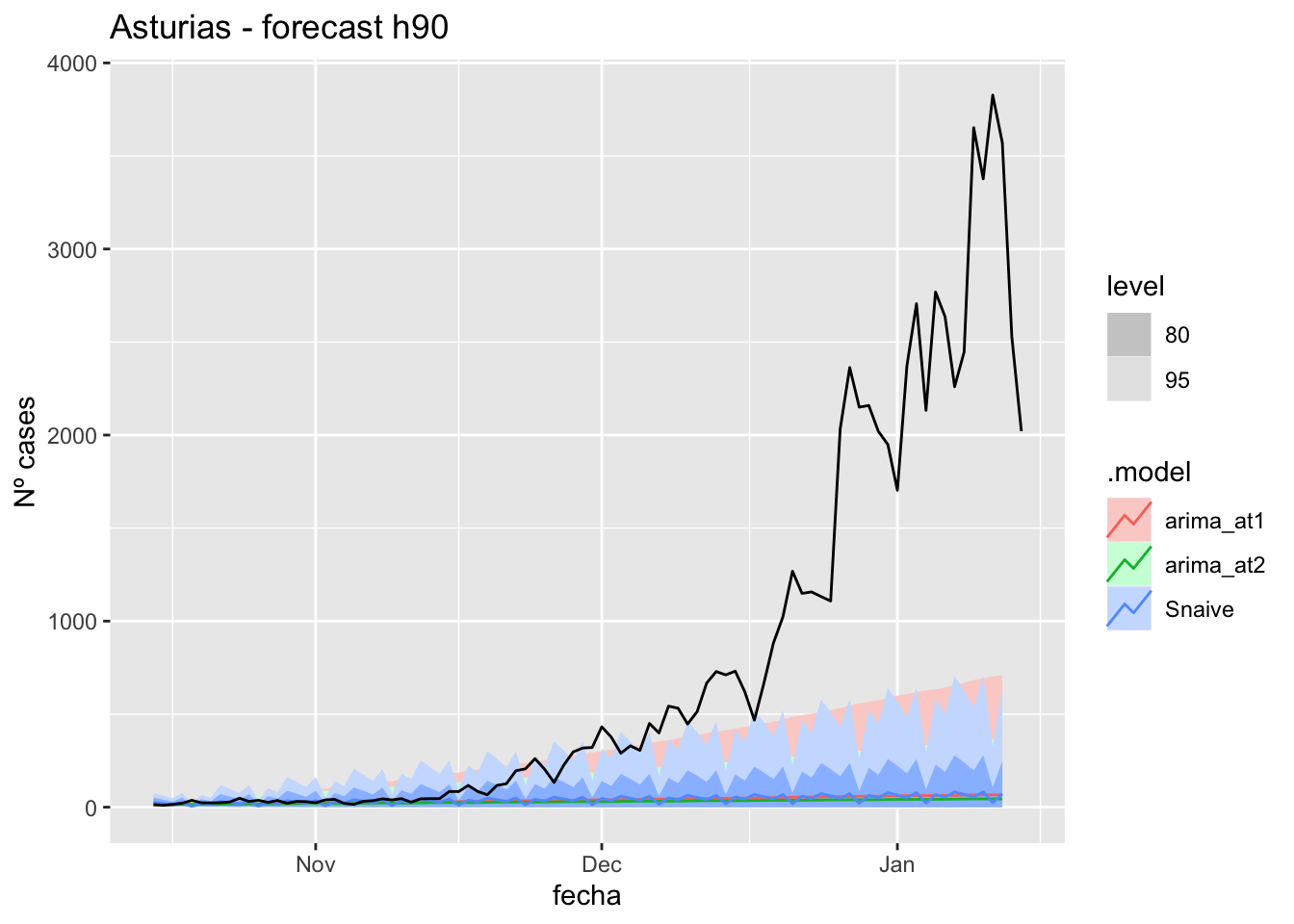
fc_h90 %>%
      autoplot(
            data_asturias %>%
                  filter(fecha <= as.Date("2021-10-14", format = "%Y-%m-%d")+days(92) &
                               fecha > as.Date("2021-07-01", format = "%Y-%m-%d"))
      ) +
      labs(y = "Nº cases", title = "Asturias - forecast h90")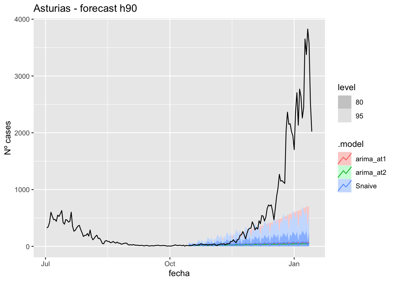
# Accuracy
fabletools::accuracy(fc_h90, data_asturias)
# A tibble: 3 × 11
.model provincia .type ME RMSE MAE MPE MAPE MASE RMSSE ACF1
<chr> <chr> <chr> <dbl> <dbl> <dbl> <dbl> <dbl> <dbl> <dbl> <dbl>
1 arima_at1 Asturias Test 704. 1211. 704. 67.5 70.0 14.2 14.8 0.925
2 arima_at2 Asturias Test 713. 1221. 714. 71.1 72.9 14.4 14.9 0.926
3 Snaive Asturias Test 702. 1213. 704. 60.0 71.7 14.2 14.8 0.925Barcelona
data_Barcelona <- covid_data %>%
      filter(provincia == "Barcelona") %>%
      filter(fecha > as.Date("2020-06-14", format = "%Y-%m-%d")) %>%
      select(provincia, fecha, num_casos, tmed) %>%
      drop_na() %>%
      as_tsibble(key = provincia, index = fecha)
data_Barcelona
# A tsibble: 653 x 4 [1D]
# Key: provincia [1]
provincia fecha num_casos tmed
<chr> <date> <dbl> <dbl>
1 Barcelona 2020-06-15 62 21.2
2 Barcelona 2020-06-16 66 20.8
3 Barcelona 2020-06-17 70 20.3
4 Barcelona 2020-06-18 68 18.8
5 Barcelona 2020-06-19 65 20.4
6 Barcelona 2020-06-20 53 21.8
7 Barcelona 2020-06-21 38 22.8
8 Barcelona 2020-06-22 69 23.8
9 Barcelona 2020-06-23 95 23.4
10 Barcelona 2020-06-24 44 23.6
# … with 643 more rowsdata_Barcelona_train <- data_Barcelona %>%
filter(fecha <= as.Date("2021-10-14", format = "%Y-%m-%d"))
summary(data_Barcelona_train$fecha) Min. 1st Qu. Median Mean 3rd Qu. Max.
"2020-06-15" "2020-10-14" "2021-02-13" "2021-02-13" "2021-06-14" "2021-10-14" data_Barcelona_test <- data_Barcelona %>%
filter(fecha > as.Date("2021-10-14", format = "%Y-%m-%d"))
summary(data_Barcelona_test$fecha) Min. 1st Qu. Median Mean 3rd Qu. Max.
"2021-10-15" "2021-11-25" "2022-01-05" "2022-01-05" "2022-02-15" "2022-03-29" # Lamba for num_casos
lambda_Barcelona_casos <- data_Barcelona %>%
features(num_casos, features = guerrero) %>%
pull(lambda_guerrero)
lambda_Barcelona_casos[1] 0.1434101# Lamba for average temp
lambda_Barcelona_tmed <- data_Barcelona %>%
features(tmed, features = guerrero) %>%
pull(lambda_guerrero)
lambda_Barcelona_tmed[1] 1.098957fit_model <- data_Barcelona_train %>%
model(
arima_at1 = ARIMA(box_cox(num_casos, lambda_Barcelona_casos) ~
box_cox(tmed, lambda_Barcelona_tmed)),
arima_at2 = ARIMA(box_cox(num_casos, lambda_Barcelona_casos) ~
box_cox(tmed, lambda_Barcelona_tmed),
stepwise = FALSE, approx = FALSE),
Snaive = SNAIVE(box_cox(num_casos, lambda_Barcelona_casos))
)
# Show and report model
fit_model# A mable: 1 x 4
# Key: provincia [1]
provincia arima_at1
<chr> <model>
1 Barcelona <LM w/ ARIMA(0,1,3)(0,1,2)[7] errors>
# … with 2 more variables: arima_at2 <model>, Snaive <model>glance(fit_model)# A tibble: 3 × 9
provincia .model sigma2 log_lik AIC AICc BIC ar_roots ma_roots
<chr> <chr> <dbl> <dbl> <dbl> <dbl> <dbl> <list> <list>
1 Barcelona arima_at1 0.195 -291. 595. 595. 624. <cpl [0]> <cpl [17]>
2 Barcelona arima_at2 0.187 -280. 575. 575. 604. <cpl [1]> <cpl [16]>
3 Barcelona Snaive 0.964 NA NA NA NA <NULL> <NULL> fit_model %>%
pivot_longer(-provincia,
names_to = ".model",
values_to = "orders") %>%
left_join(glance(fit_model), by = c("provincia", ".model")) %>%
arrange(AICc) %>%
select(.model:BIC)# A mable: 3 x 7
# Key: .model [3]
.model orders sigma2 log_lik AIC AICc BIC
<chr> <model> <dbl> <dbl> <dbl> <dbl> <dbl>
1 arima_… <LM w/ ARIMA(1,1,2)(0,1,2)[7] errors> 0.187 -280. 575. 575. 604.
2 arima_… <LM w/ ARIMA(0,1,3)(0,1,2)[7] errors> 0.195 -291. 595. 595. 624.
3 Snaive <SNAIVE> 0.964 NA NA NA NA # We use a Ljung-Box test >> large p-value, confirms residuals are similar / considered to white noise
fit_model %>%
select(Snaive) %>%
gg_tsresiduals()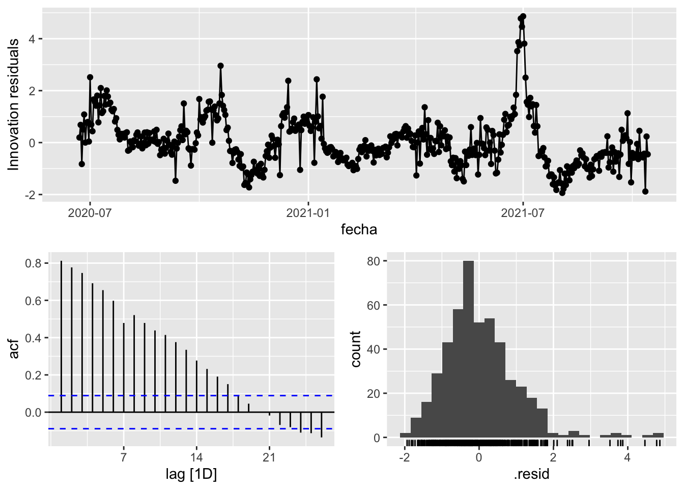
fit_model %>%
      select(arima_at1) %>%
      gg_tsresiduals()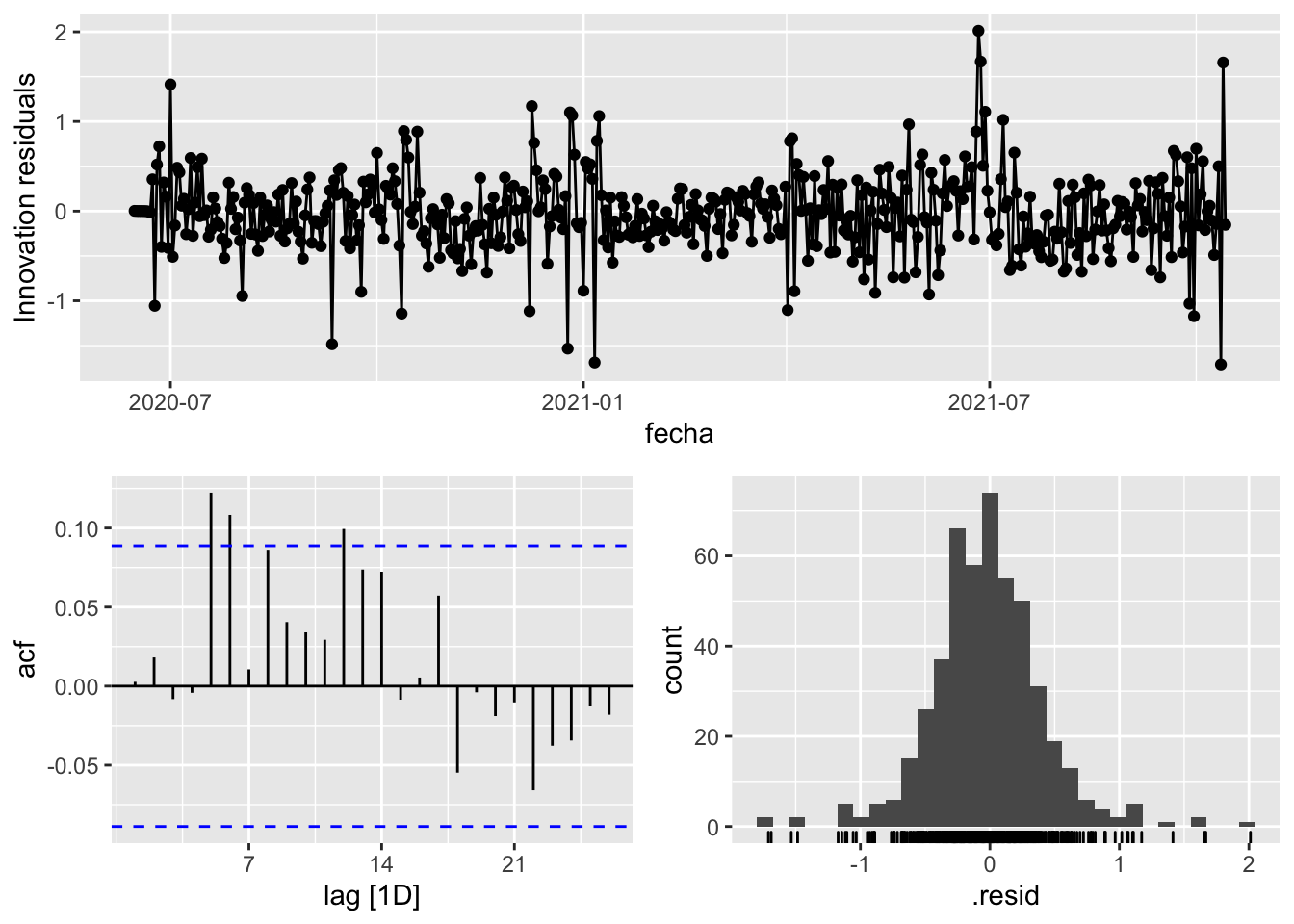
fit_model %>%
      select(arima_at2) %>%
      gg_tsresiduals()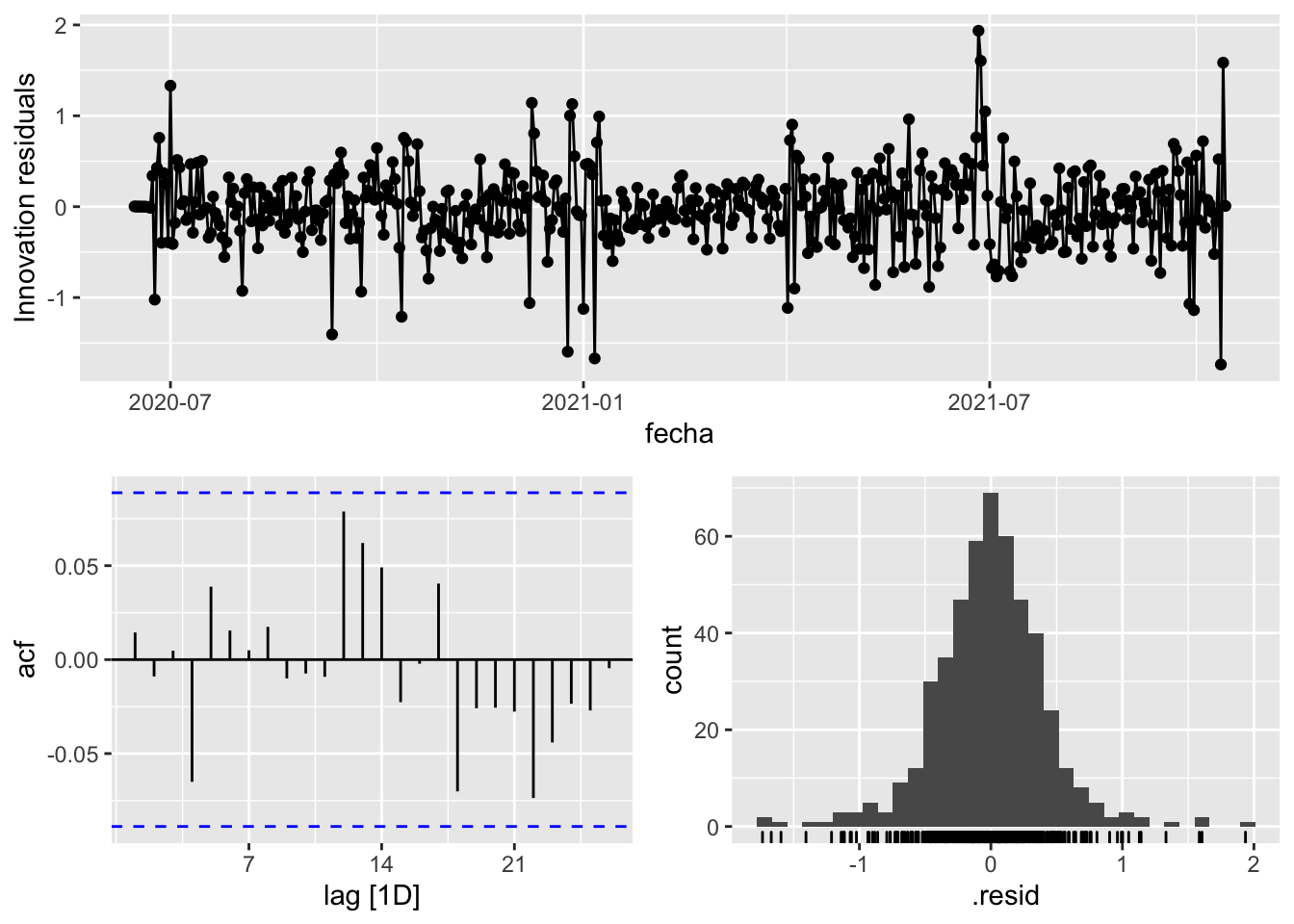
augment(fit_model) %>%
      features(.innov, ljung_box, lag=7)
# A tibble: 3 × 4
provincia .model lb_stat lb_pvalue
<chr> <chr> <dbl> <dbl>
1 Barcelona arima_at1 13.5 0.0615
2 Barcelona arima_at2 3.11 0.874
3 Barcelona Snaive 1610. 0 augment(fit_model) %>%
features(.innov, ljung_box, lag=14)# A tibble: 3 × 4
provincia .model lb_stat lb_pvalue
<chr> <chr> <dbl> <dbl>
1 Barcelona arima_at1 29.3 0.00944
2 Barcelona arima_at2 9.65 0.787
3 Barcelona Snaive 2198. 0 augment(fit_model) %>%
features(.innov, ljung_box, lag=21)# A tibble: 3 × 4
provincia .model lb_stat lb_pvalue
<chr> <chr> <dbl> <dbl>
1 Barcelona arima_at1 32.8 0.0484
2 Barcelona arima_at2 14.3 0.856
3 Barcelona Snaive 2259. 0 augment(fit_model) %>%
features(.innov, ljung_box, lag=90)# A tibble: 3 × 4
provincia .model lb_stat lb_pvalue
<chr> <chr> <dbl> <dbl>
1 Barcelona arima_at1 133. 0.00214
2 Barcelona arima_at2 86.8 0.576
3 Barcelona Snaive 3453. 0 # To predict future values of infections, we need to pass the model future/prediction values of the complementary variables tmed and mobility
# We are going to select those from the test dataset
data_fc_h7 <- data_Barcelona_test %>%
select(-num_casos) %>%
slice(1:7)
data_fc_h14 <- data_Barcelona_test %>%
select(-num_casos) %>%
slice(1:14)
data_fc_h21 <- data_Barcelona_test %>%
select(-num_casos) %>%
slice(1:21)
data_fc_h90 <- data_Barcelona_test %>%
select(-num_casos) %>%
slice(1:90)# Significant spikes out of 30 is still consistent with white noise
# To be sure, use a Ljung-Box test, which has a large p-value, confirming that
# the residuals are similar to white noise.
# Note that the alternative models also passed this test.
#
# Forecast
fc_h7 <- fabletools::forecast(fit_model, new_data = data_fc_h7)
fc_h14 <- fabletools::forecast(fit_model, new_data = data_fc_h14)
fc_h21 <- fabletools::forecast(fit_model, new_data = data_fc_h21)
fc_h90 <- fabletools::forecast(fit_model, new_data = data_fc_h90)7 days
# Plots
fc_h7 %>%
      autoplot(
            data_Barcelona_test %>%
                  filter(fecha <= as.Date("2021-10-14", format = "%Y-%m-%d")+days(9))
      ) +
      labs(y = "Nº cases", title = "Barcelona - forecast h7")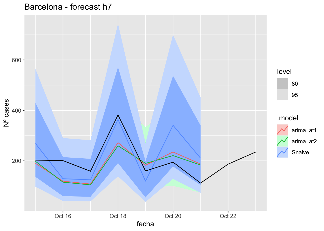
fc_h7 %>%
      autoplot(
            data_Barcelona %>%
                  filter(fecha <= as.Date("2021-10-14", format = "%Y-%m-%d")+days(9) &
                               fecha > as.Date("2021-07-01", format = "%Y-%m-%d"))
      ) +
      labs(y = "Nº cases", title = "Barcelona - forecast h7")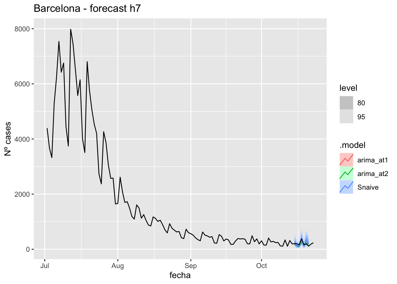
# Accuracy
fabletools::accuracy(fc_h7, data_Barcelona)
# A tibble: 3 × 11
.model provincia .type ME RMSE MAE MPE MAPE MASE RMSSE ACF1
<chr> <chr> <chr> <dbl> <dbl> <dbl> <dbl> <dbl> <dbl> <dbl> <dbl>
1 arima_at1 Barcelona Test 16.6 64.7 56.2 0.729 30.0 0.149 0.0975 0.327
2 arima_at2 Barcelona Test 19.8 67.5 56.3 2.11 29.6 0.150 0.102 0.211
3 Snaive Barcelona Test -21.0 79.0 67.8 -15.5 40.3 0.180 0.119 0.18414 days
# Plots
fc_h14 %>%
      autoplot(
            data_Barcelona_test %>%
                  filter(fecha <= as.Date("2021-10-14", format = "%Y-%m-%d")+days(16))
      ) +
      labs(y = "Nº cases", title = "Barcelona - forecast h14")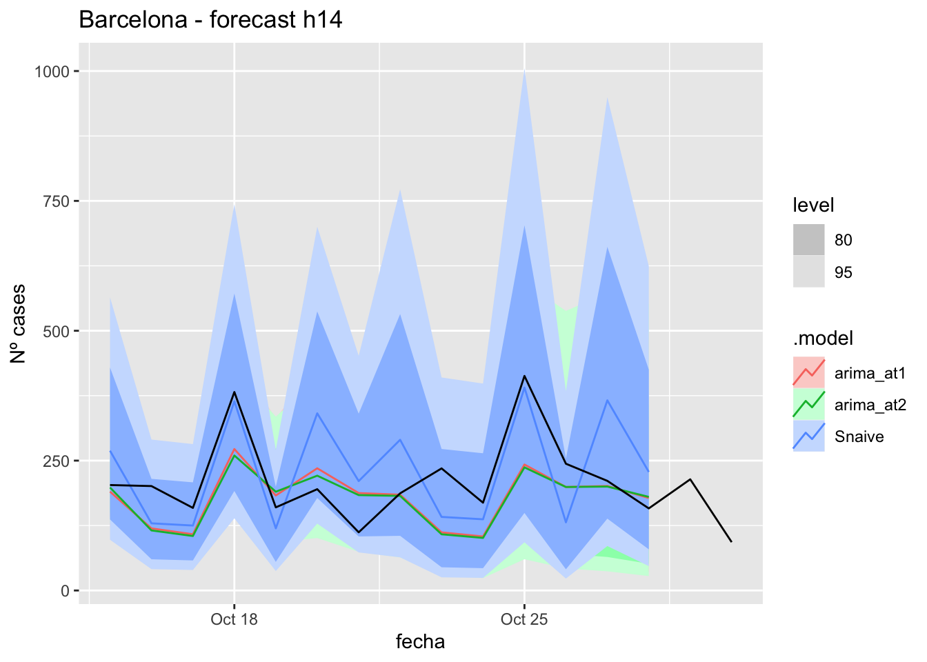
fc_h14 %>%
      autoplot(
            data_Barcelona %>%
                  filter(fecha <= as.Date("2021-10-14", format = "%Y-%m-%d")+days(16) &
                               fecha > as.Date("2021-07-01", format = "%Y-%m-%d"))
      ) +
      labs(y = "Nº cases", title = "Barcelona - forecast h14")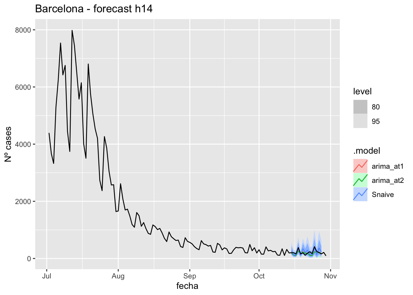
# Accuracy
fabletools::accuracy(fc_h14, data_Barcelona)
# A tibble: 3 × 11
.model provincia .type ME RMSE MAE MPE MAPE MASE RMSSE ACF1
<chr> <chr> <chr> <dbl> <dbl> <dbl> <dbl> <dbl> <dbl> <dbl> <dbl>
1 arima_at1 Barcelona Test 36.6 75.7 59.2 10.6 27.1 0.157 0.114 0.308
2 arima_at2 Barcelona Test 39.1 78.5 60.5 11.7 27.4 0.161 0.118 0.245
3 Snaive Barcelona Test -15.3 87.1 76.0 -12.2 40.4 0.202 0.131 0.061021 days
# Plots
fc_h21 %>%
      autoplot(
            data_Barcelona_test %>%
                  filter(fecha <= as.Date("2021-10-14", format = "%Y-%m-%d")+days(23))
      ) +
      labs(y = "Nº cases", title = "Barcelona - forecast h21")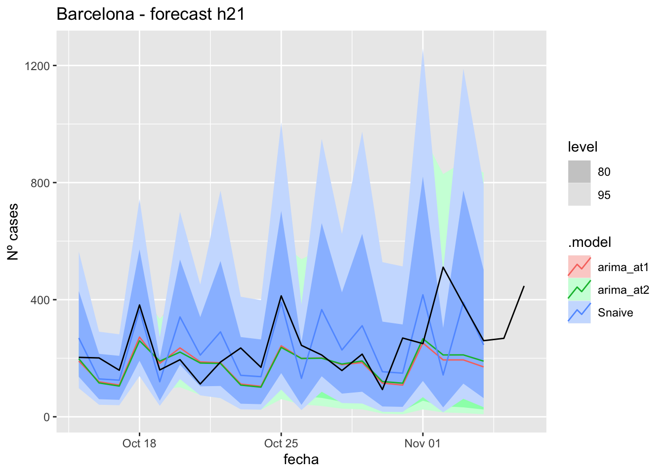
fc_h21 %>%
      autoplot(
            data_Barcelona %>%
                  filter(fecha <= as.Date("2021-10-14", format = "%Y-%m-%d")+days(23) &
                               fecha > as.Date("2021-07-01", format = "%Y-%m-%d"))
      ) +
      labs(y = "Nº cases", title = "Barcelona - forecast h21")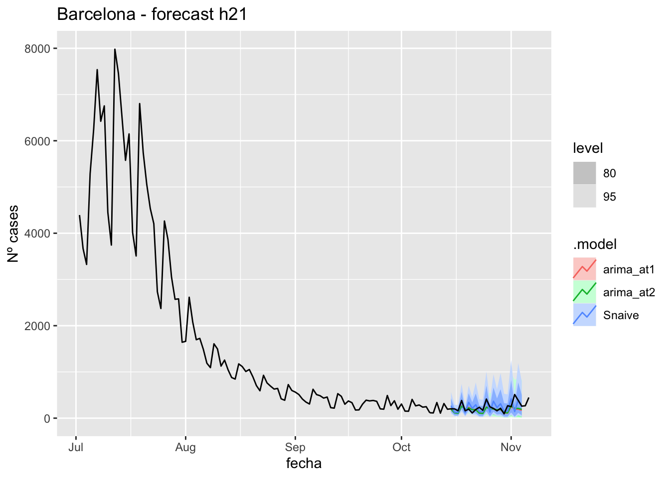
# Accuracy
fabletools::accuracy(fc_h21, data_Barcelona)
# A tibble: 3 × 11
.model provincia .type ME RMSE MAE MPE MAPE MASE RMSSE ACF1
<chr> <chr> <chr> <dbl> <dbl> <dbl> <dbl> <dbl> <dbl> <dbl> <dbl>
1 arima_at1 Barcelona Test 60.6 109. 78.0 16.3 29.7 0.207 0.165 0.206
2 arima_at2 Barcelona Test 58.3 106. 76.7 15.5 29.5 0.204 0.160 0.122
3 Snaive Barcelona Test -2.10 119. 90.4 -10.9 41.3 0.240 0.179 -0.23990 days
# Plots
fc_h90 %>%
      autoplot(
            data_Barcelona_test %>%
                  filter(fecha <= as.Date("2021-10-14", format = "%Y-%m-%d")+days(92))
      ) +
      labs(y = "Nº cases", title = "Barcelona - forecast h90")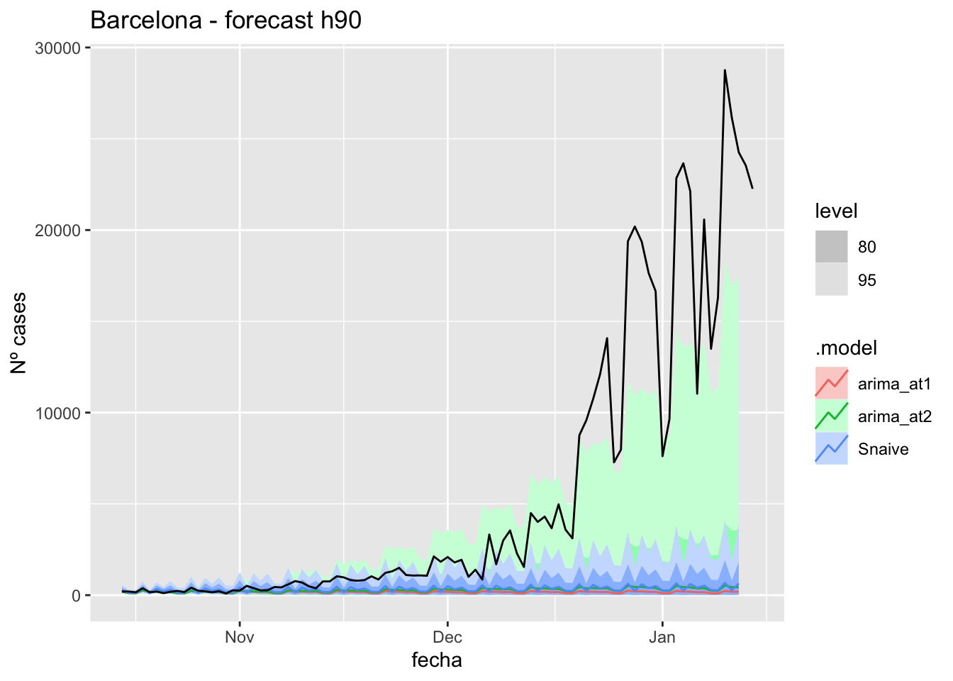
fc_h90 %>%
      autoplot(
            data_Barcelona %>%
                  filter(fecha <= as.Date("2021-10-14", format = "%Y-%m-%d")+days(92) &
                               fecha > as.Date("2021-07-01", format = "%Y-%m-%d"))
      ) +
      labs(y = "Nº cases", title = "Barcelona - forecast h90")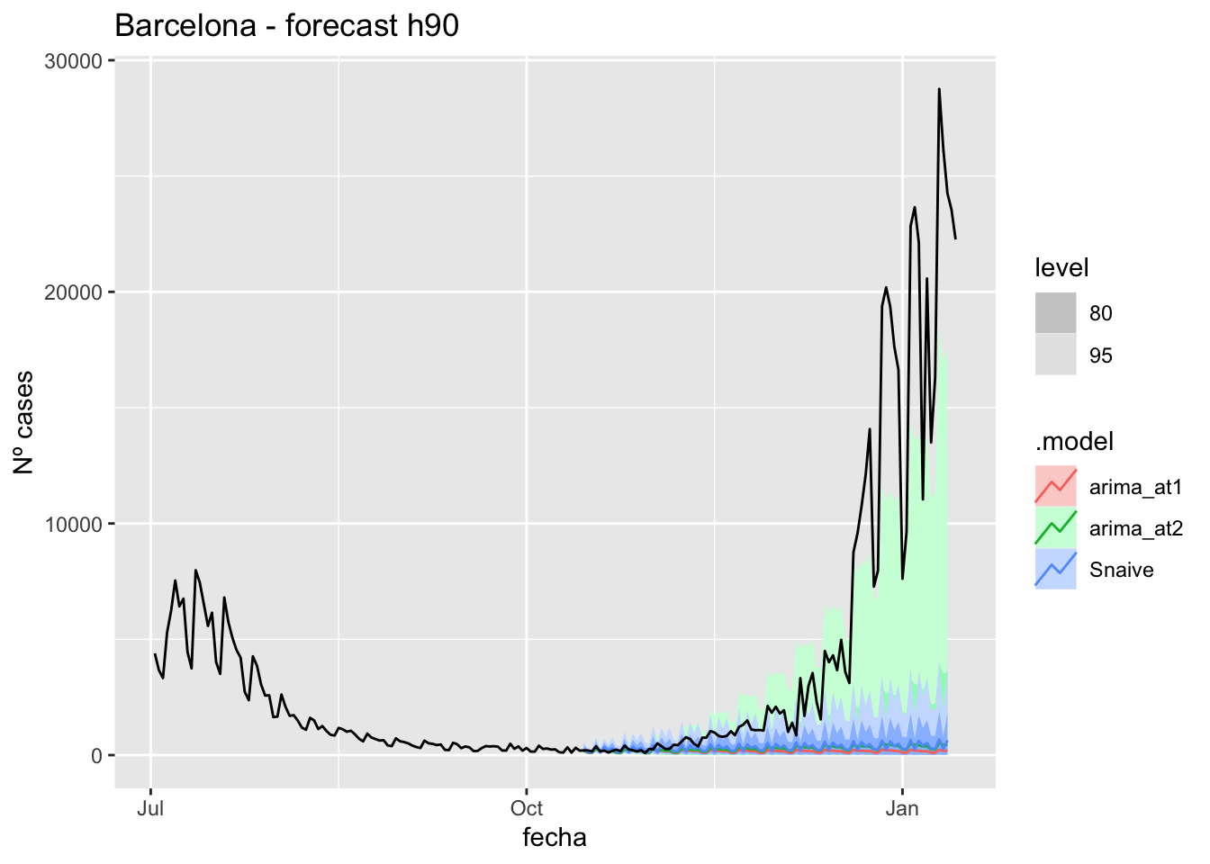
# Accuracy
fabletools::accuracy(fc_h90, data_Barcelona)
# A tibble: 3 × 11
.model provincia .type ME RMSE MAE MPE MAPE MASE RMSSE ACF1
<chr> <chr> <chr> <dbl> <dbl> <dbl> <dbl> <dbl> <dbl> <dbl> <dbl>
1 arima_at1 Barcelona Test 5077. 9032. 5081. 72.5 75.6 13.5 13.6 0.868
2 arima_at2 Barcelona Test 4972. 8914. 4977. 68.6 71.8 13.2 13.4 0.868
3 Snaive Barcelona Test 4916. 8890. 4939. 58.7 71.4 13.1 13.4 0.870Madrid
data_Madrid <- covid_data %>%
      filter(provincia == "Madrid") %>%
      filter(fecha > as.Date("2020-06-14", format = "%Y-%m-%d")) %>%
      select(provincia, fecha, num_casos, tmed) %>%
      drop_na() %>%
      as_tsibble(key = provincia, index = fecha)
data_Madrid
# A tsibble: 653 x 4 [1D]
# Key: provincia [1]
provincia fecha num_casos tmed
<chr> <date> <dbl> <dbl>
1 Madrid 2020-06-15 153 20.7
2 Madrid 2020-06-16 91 21
3 Madrid 2020-06-17 93 20.2
4 Madrid 2020-06-18 85 21.9
5 Madrid 2020-06-19 78 22.6
6 Madrid 2020-06-20 67 23.4
7 Madrid 2020-06-21 42 25
8 Madrid 2020-06-22 60 27.3
9 Madrid 2020-06-23 68 28.4
10 Madrid 2020-06-24 49 28
# … with 643 more rowsdata_Madrid_train <- data_Madrid %>%
filter(fecha <= as.Date("2021-10-14", format = "%Y-%m-%d"))
summary(data_Madrid_train$fecha) Min. 1st Qu. Median Mean 3rd Qu. Max.
"2020-06-15" "2020-10-14" "2021-02-13" "2021-02-13" "2021-06-14" "2021-10-14" data_Madrid_test <- data_Madrid %>%
filter(fecha > as.Date("2021-10-14", format = "%Y-%m-%d"))
summary(data_Madrid_test$fecha) Min. 1st Qu. Median Mean 3rd Qu. Max.
"2021-10-15" "2021-11-25" "2022-01-05" "2022-01-05" "2022-02-15" "2022-03-29" # Lamba for num_casos
lambda_Madrid_casos <- data_Madrid %>%
features(num_casos, features = guerrero) %>%
pull(lambda_guerrero)
lambda_Madrid_casos[1] 0.06260614# Lamba for average temp
lambda_Madrid_tmed <- data_Madrid %>%
features(tmed, features = guerrero) %>%
pull(lambda_guerrero)
lambda_Madrid_tmed[1] 0.936519fit_model <- data_Madrid_train %>%
model(
arima_at1 = ARIMA(box_cox(num_casos, lambda_Madrid_casos) ~
box_cox(tmed, lambda_Madrid_tmed)),
arima_at2 = ARIMA(box_cox(num_casos, lambda_Madrid_casos) ~
box_cox(tmed, lambda_Madrid_tmed),
stepwise = FALSE, approx = FALSE),
Snaive = SNAIVE(box_cox(num_casos, lambda_Madrid_casos))
)
# Show and report model
fit_model# A mable: 1 x 4
# Key: provincia [1]
provincia arima_at1
<chr> <model>
1 Madrid <LM w/ ARIMA(2,1,1)(1,1,1)[7] errors>
# … with 2 more variables: arima_at2 <model>, Snaive <model>glance(fit_model)# A tibble: 3 × 9
provincia .model sigma2 log_lik AIC AICc BIC ar_roots ma_roots
<chr> <chr> <dbl> <dbl> <dbl> <dbl> <dbl> <list> <list>
1 Madrid arima_at1 0.0669 -33.4 80.8 81.1 110. <cpl [9]> <cpl [8]>
2 Madrid arima_at2 0.0669 -33.4 80.8 81.1 110. <cpl [9]> <cpl [8]>
3 Madrid Snaive 0.291 NA NA NA NA <NULL> <NULL> fit_model %>%
pivot_longer(-provincia,
names_to = ".model",
values_to = "orders") %>%
left_join(glance(fit_model), by = c("provincia", ".model")) %>%
arrange(AICc) %>%
select(.model:BIC)# A mable: 3 x 7
# Key: .model [3]
.model orders sigma2 log_lik AIC AICc BIC
<chr> <model> <dbl> <dbl> <dbl> <dbl> <dbl>
1 arima_… <LM w/ ARIMA(2,1,1)(1,1,1)[7] errors> 0.0669 -33.4 80.8 81.1 110.
2 arima_… <LM w/ ARIMA(2,1,1)(1,1,1)[7] errors> 0.0669 -33.4 80.8 81.1 110.
3 Snaive <SNAIVE> 0.291 NA NA NA NA # We use a Ljung-Box test >> large p-value, confirms residuals are similar / considered to white noise
fit_model %>%
select(Snaive) %>%
gg_tsresiduals()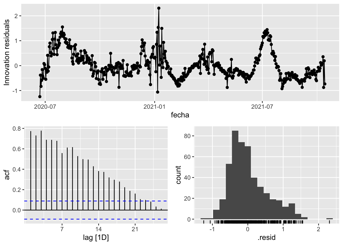
fit_model %>%
      select(arima_at1) %>%
      gg_tsresiduals()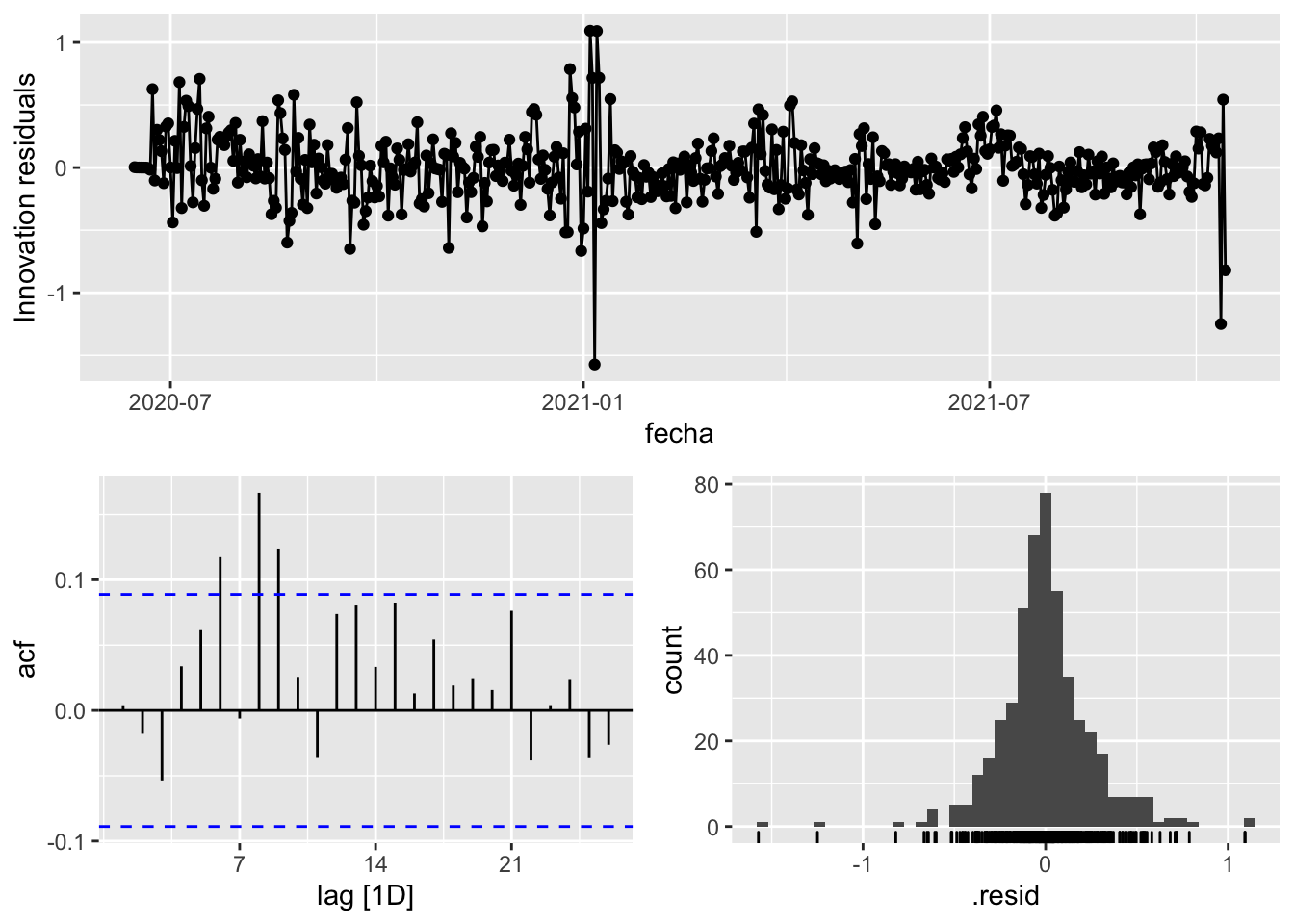
fit_model %>%
      select(arima_at2) %>%
      gg_tsresiduals()
augment(fit_model) %>%
      features(.innov, ljung_box, lag=7)
# A tibble: 3 × 4
provincia .model lb_stat lb_pvalue
<chr> <chr> <dbl> <dbl>
1 Madrid arima_at1 10.8 0.146
2 Madrid arima_at2 10.8 0.146
3 Madrid Snaive 1678. 0 augment(fit_model) %>%
features(.innov, ljung_box, lag=14)# A tibble: 3 × 4
provincia .model lb_stat lb_pvalue
<chr> <chr> <dbl> <dbl>
1 Madrid arima_at1 39.8 0.000272
2 Madrid arima_at2 39.8 0.000272
3 Madrid Snaive 2594. 0 augment(fit_model) %>%
features(.innov, ljung_box, lag=21)# A tibble: 3 × 4
provincia .model lb_stat lb_pvalue
<chr> <chr> <dbl> <dbl>
1 Madrid arima_at1 48.4 0.000605
2 Madrid arima_at2 48.4 0.000605
3 Madrid Snaive 2854. 0 augment(fit_model) %>%
features(.innov, ljung_box, lag=90)# A tibble: 3 × 4
provincia .model lb_stat lb_pvalue
<chr> <chr> <dbl> <dbl>
1 Madrid arima_at1 106. 0.126
2 Madrid arima_at2 106. 0.126
3 Madrid Snaive 3856. 0 # To predict future values of infections, we need to pass the model future/prediction values of the complementary variables tmed and mobility
# We are going to select those from the test dataset
data_fc_h7 <- data_Madrid_test %>%
select(-num_casos) %>%
slice(1:7)
data_fc_h14 <- data_Madrid_test %>%
select(-num_casos) %>%
slice(1:14)
data_fc_h21 <- data_Madrid_test %>%
select(-num_casos) %>%
slice(1:21)
data_fc_h90 <- data_Madrid_test %>%
select(-num_casos) %>%
slice(1:90)# Significant spikes out of 30 is still consistent with white noise
# To be sure, use a Ljung-Box test, which has a large p-value, confirming that
# the residuals are similar to white noise.
# Note that the alternative models also passed this test.
#
# Forecast
fc_h7 <- fabletools::forecast(fit_model, new_data = data_fc_h7)
fc_h14 <- fabletools::forecast(fit_model, new_data = data_fc_h14)
fc_h21 <- fabletools::forecast(fit_model, new_data = data_fc_h21)
fc_h90 <- fabletools::forecast(fit_model, new_data = data_fc_h90)7 days
# Plots
fc_h7 %>%
      autoplot(
            data_Madrid_test %>%
                  filter(fecha <= as.Date("2021-10-14", format = "%Y-%m-%d")+days(9))
      ) +
      labs(y = "Nº cases", title = "Madrid - forecast h7")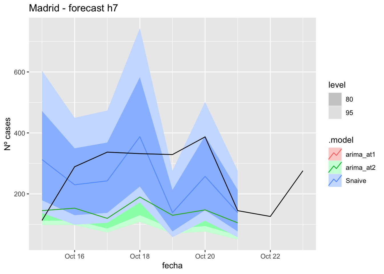
fc_h7 %>%
      autoplot(
            data_Madrid %>%
                  filter(fecha <= as.Date("2021-10-14", format = "%Y-%m-%d")+days(9) &
                               fecha > as.Date("2021-07-01", format = "%Y-%m-%d"))
      ) +
      labs(y = "Nº cases", title = "Madrid - forecast h7")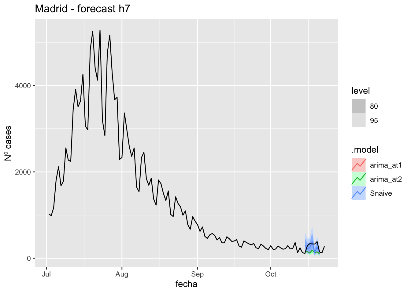
# Accuracy
fabletools::accuracy(fc_h7, data_Madrid)
# A tibble: 3 × 11
.model provincia .type ME RMSE MAE MPE MAPE MASE RMSSE ACF1
<chr> <chr> <chr> <dbl> <dbl> <dbl> <dbl> <dbl> <dbl> <dbl> <dbl>
1 arima_at1 Madrid Test 135. 163. 144. 39.4 47.5 0.339 0.242 -0.0363
2 arima_at2 Madrid Test 135. 163. 144. 39.4 47.5 0.339 0.242 -0.0363
3 Snaive Madrid Test 32.1 124. 105. -7.03 48.2 0.247 0.185 -0.109 14 days
# Plots
fc_h14 %>%
      autoplot(
            data_Madrid_test %>%
                  filter(fecha <= as.Date("2021-10-14", format = "%Y-%m-%d")+days(16))
      ) +
      labs(y = "Nº cases", title = "Madrid - forecast h14")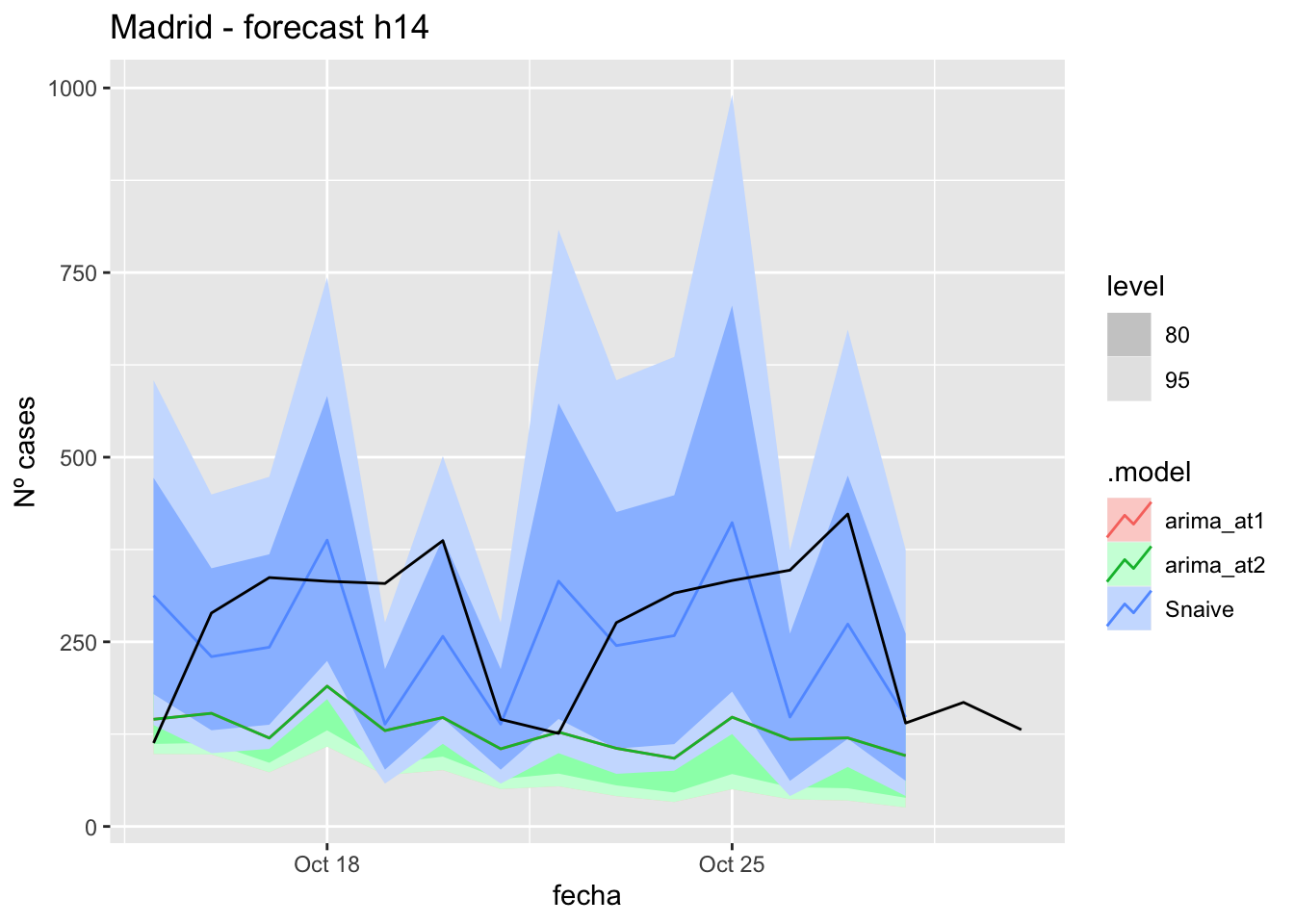
fc_h14 %>%
      autoplot(
            data_Madrid %>%
                  filter(fecha <= as.Date("2021-10-14", format = "%Y-%m-%d")+days(16) &
                               fecha > as.Date("2021-07-01", format = "%Y-%m-%d"))
      ) +
      labs(y = "Nº cases", title = "Madrid - forecast h14")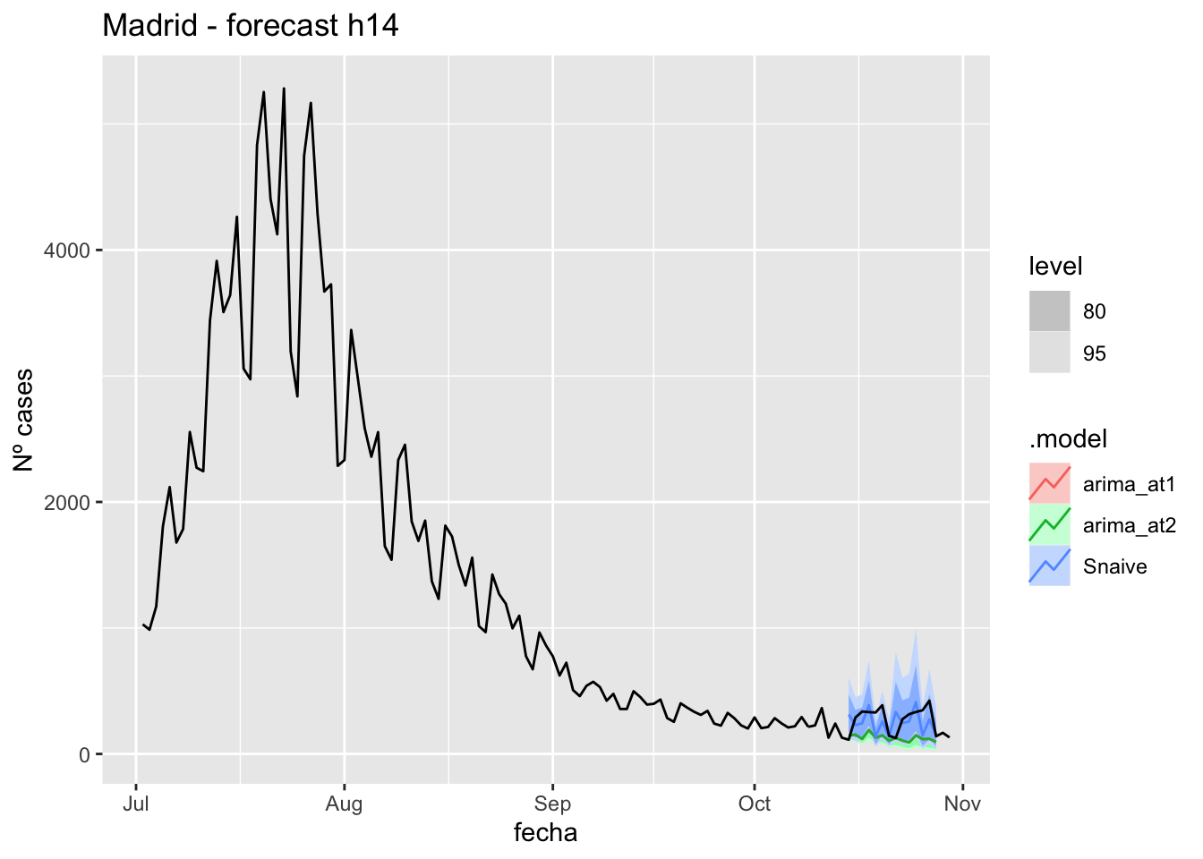
# Accuracy
fabletools::accuracy(fc_h14, data_Madrid)
# A tibble: 3 × 11
.model provincia .type ME RMSE MAE MPE MAPE MASE RMSSE ACF1
<chr> <chr> <chr> <dbl> <dbl> <dbl> <dbl> <dbl> <dbl> <dbl> <dbl>
1 arima_at1 Madrid Test 150. 178. 154. 45.1 49.4 0.364 0.265 0.0893
2 arima_at2 Madrid Test 150. 178. 154. 45.1 49.4 0.364 0.265 0.0893
3 Snaive Madrid Test 26.3 126. 105. -8.58 46.6 0.246 0.188 -0.047221 days
# Plots
fc_h21 %>%
      autoplot(
            data_Madrid_test %>%
                  filter(fecha <= as.Date("2021-10-14", format = "%Y-%m-%d")+days(23))
      ) +
      labs(y = "Nº cases", title = "Madrid - forecast h21")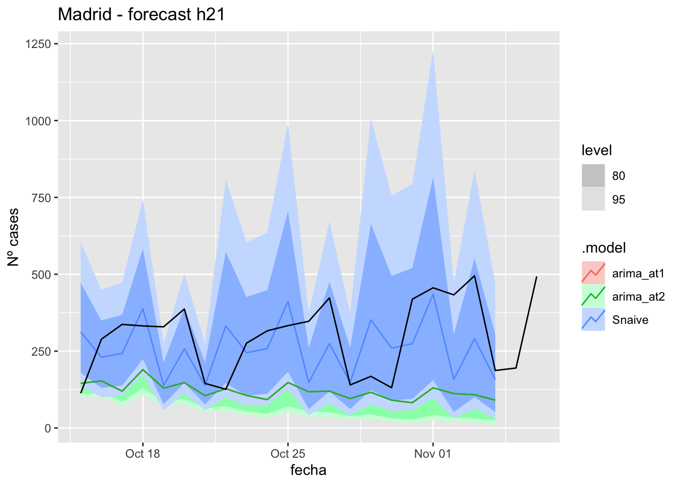
fc_h21 %>%
      autoplot(
            data_Madrid %>%
                  filter(fecha <= as.Date("2021-10-14", format = "%Y-%m-%d")+days(23) &
                               fecha > as.Date("2021-07-01", format = "%Y-%m-%d"))
      ) +
      labs(y = "Nº cases", title = "Madrid - forecast h21")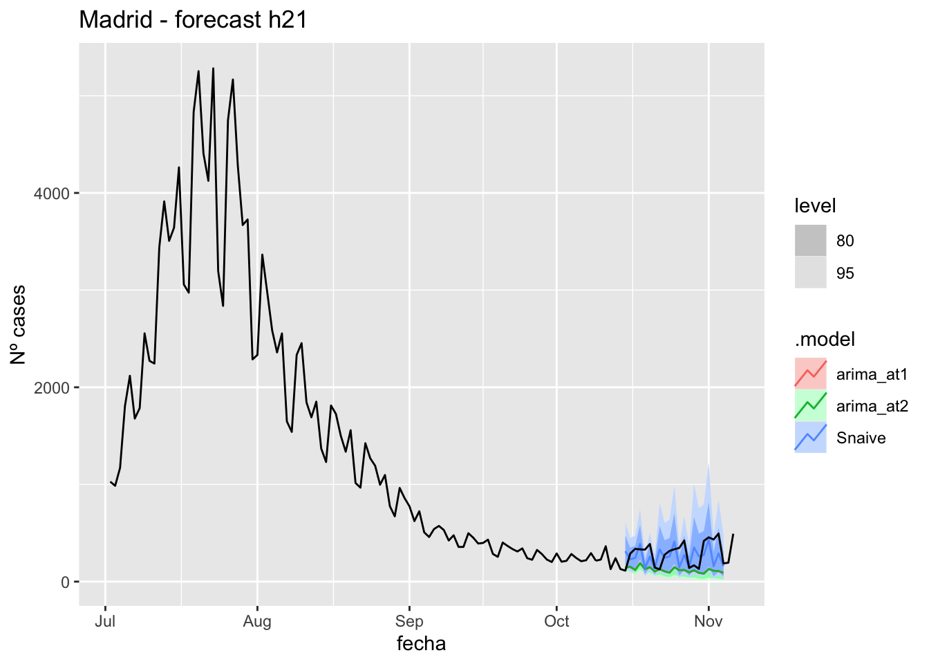
# Accuracy
fabletools::accuracy(fc_h21, data_Madrid)
# A tibble: 3 × 11
.model provincia .type ME RMSE MAE MPE MAPE MASE RMSSE ACF1
<chr> <chr> <chr> <dbl> <dbl> <dbl> <dbl> <dbl> <dbl> <dbl> <dbl>
1 arima_at1 Madrid Test 174. 210. 177. 50.0 52.8 0.418 0.313 0.287
2 arima_at2 Madrid Test 174. 210. 177. 50.0 52.8 0.418 0.313 0.287
3 Snaive Madrid Test 34.8 140. 117. -8.01 48.6 0.275 0.209 0.13190 days
# Plots
fc_h90 %>%
      autoplot(
            data_Madrid_test %>%
                  filter(fecha <= as.Date("2021-10-14", format = "%Y-%m-%d")+days(92))
      ) +
      labs(y = "Nº cases", title = "Madrid - forecast h90")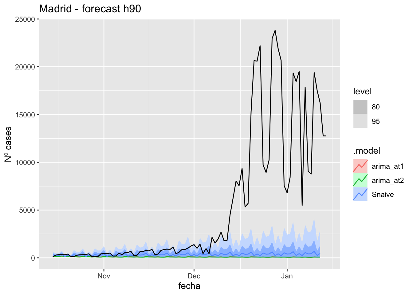
fc_h90 %>%
      autoplot(
            data_Madrid %>%
                  filter(fecha <= as.Date("2021-10-14", format = "%Y-%m-%d")+days(92) &
                               fecha > as.Date("2021-07-01", format = "%Y-%m-%d"))
      ) +
      labs(y = "Nº cases", title = "Madrid - forecast h90")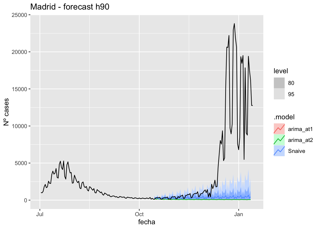
# Accuracy
fabletools::accuracy(fc_h90, data_Madrid)
# A tibble: 3 × 11
.model provincia .type ME RMSE MAE MPE MAPE MASE RMSSE ACF1
<chr> <chr> <chr> <dbl> <dbl> <dbl> <dbl> <dbl> <dbl> <dbl> <dbl>
1 arima_at1 Madrid Test 5007. 8744. 5008. 81.8 82.4 11.8 13.0 0.840
2 arima_at2 Madrid Test 5007. 8744. 5008. 81.8 82.4 11.8 13.0 0.840
3 Snaive Madrid Test 4763. 8564. 4792. 51.8 68.9 11.3 12.7 0.840Malaga
data_Malaga <- covid_data %>%
      filter(provincia == "Málaga") %>%
      filter(fecha > as.Date("2020-06-14", format = "%Y-%m-%d")) %>%
      select(provincia, fecha, num_casos, tmed) %>%
      drop_na() %>%
      as_tsibble(key = provincia, index = fecha)
data_Malaga
# A tsibble: 653 x 4 [1D]
# Key: provincia [1]
provincia fecha num_casos tmed
<chr> <date> <dbl> <dbl>
1 Málaga 2020-06-15 1 27.2
2 Málaga 2020-06-16 1 27.8
3 Málaga 2020-06-17 2 26.9
4 Málaga 2020-06-18 2 21.6
5 Málaga 2020-06-19 1 24.7
6 Málaga 2020-06-20 4 22.6
7 Málaga 2020-06-21 4 22.7
8 Málaga 2020-06-22 6 25
9 Málaga 2020-06-23 8 25.6
10 Málaga 2020-06-24 65 24.5
# … with 643 more rowsdata_Malaga_train <- data_Malaga %>%
filter(fecha <= as.Date("2021-10-14", format = "%Y-%m-%d"))
summary(data_Malaga_train$fecha) Min. 1st Qu. Median Mean 3rd Qu. Max.
"2020-06-15" "2020-10-14" "2021-02-13" "2021-02-13" "2021-06-14" "2021-10-14" data_Malaga_test <- data_Malaga %>%
filter(fecha > as.Date("2021-10-14", format = "%Y-%m-%d"))
summary(data_Malaga_test$fecha) Min. 1st Qu. Median Mean 3rd Qu. Max.
"2021-10-15" "2021-11-25" "2022-01-05" "2022-01-05" "2022-02-15" "2022-03-29" # Lamba for num_casos
lambda_Malaga_casos <- data_Malaga %>%
features(num_casos, features = guerrero) %>%
pull(lambda_guerrero)
lambda_Malaga_casos[1] 0.2312255# Lamba for average temp
lambda_Malaga_tmed <- data_Malaga %>%
features(tmed, features = guerrero) %>%
pull(lambda_guerrero)
lambda_Malaga_tmed[1] 0.6288527fit_model <- data_Malaga_train %>%
model(
arima_at1 = ARIMA(box_cox(num_casos, lambda_Malaga_casos) ~
box_cox(tmed, lambda_Malaga_tmed)),
arima_at2 = ARIMA(box_cox(num_casos, lambda_Malaga_casos) ~
box_cox(tmed, lambda_Malaga_tmed),
stepwise = FALSE, approx = FALSE),
Snaive = SNAIVE(box_cox(num_casos, lambda_Malaga_casos))
)
# Show and report model
fit_model# A mable: 1 x 4
# Key: provincia [1]
provincia arima_at1
<chr> <model>
1 Málaga <LM w/ ARIMA(4,1,0)(2,0,0)[7] errors>
# … with 2 more variables: arima_at2 <model>, Snaive <model>glance(fit_model)# A tibble: 3 × 9
provincia .model sigma2 log_lik AIC AICc BIC ar_roots ma_roots
<chr> <chr> <dbl> <dbl> <dbl> <dbl> <dbl> <list> <list>
1 Málaga arima_at1 0.553 -545. 1105. 1105. 1139. <cpl [18]> <cpl [0]>
2 Málaga arima_at2 0.550 -543. 1102. 1103. 1136. <cpl [14]> <cpl [4]>
3 Málaga Snaive 2.15 NA NA NA NA <NULL> <NULL> fit_model %>%
pivot_longer(-provincia,
names_to = ".model",
values_to = "orders") %>%
left_join(glance(fit_model), by = c("provincia", ".model")) %>%
arrange(AICc) %>%
select(.model:BIC)# A mable: 3 x 7
# Key: .model [3]
.model orders sigma2 log_lik AIC AICc BIC
<chr> <model> <dbl> <dbl> <dbl> <dbl> <dbl>
1 arima_… <LM w/ ARIMA(0,1,4)(2,0,0)[7] errors> 0.550 -543. 1102. 1103. 1136.
2 arima_… <LM w/ ARIMA(4,1,0)(2,0,0)[7] errors> 0.553 -545. 1105. 1105. 1139.
3 Snaive <SNAIVE> 2.15 NA NA NA NA # We use a Ljung-Box test >> large p-value, confirms residuals are similar / considered to white noise
fit_model %>%
select(Snaive) %>%
gg_tsresiduals()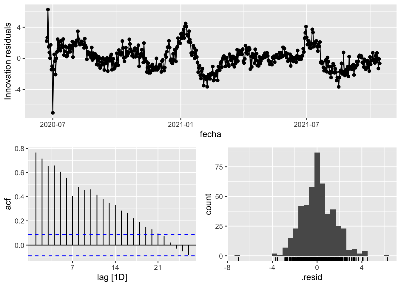
fit_model %>%
      select(arima_at1) %>%
      gg_tsresiduals()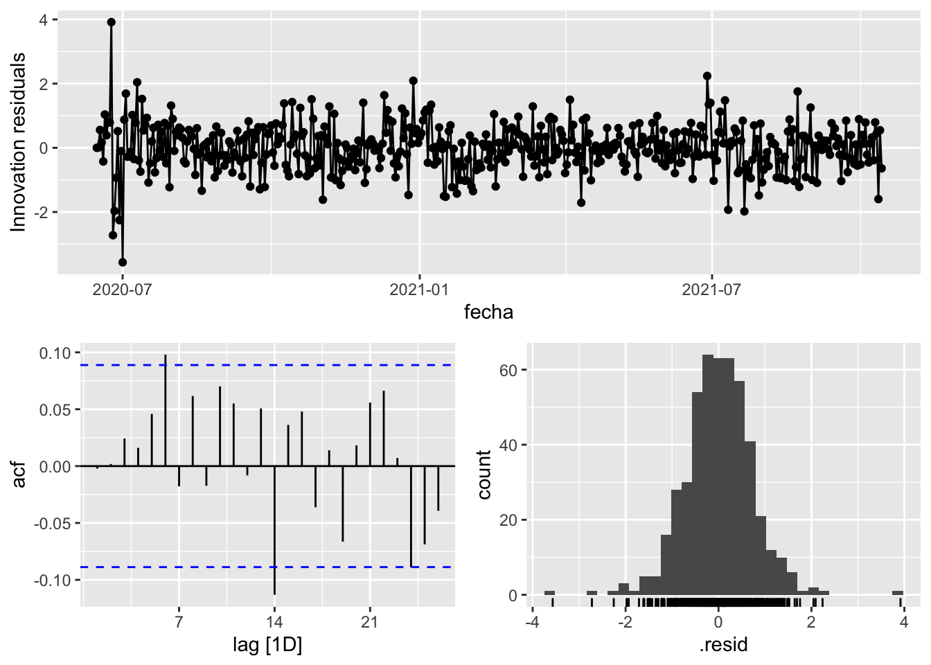
fit_model %>%
      select(arima_at2) %>%
      gg_tsresiduals()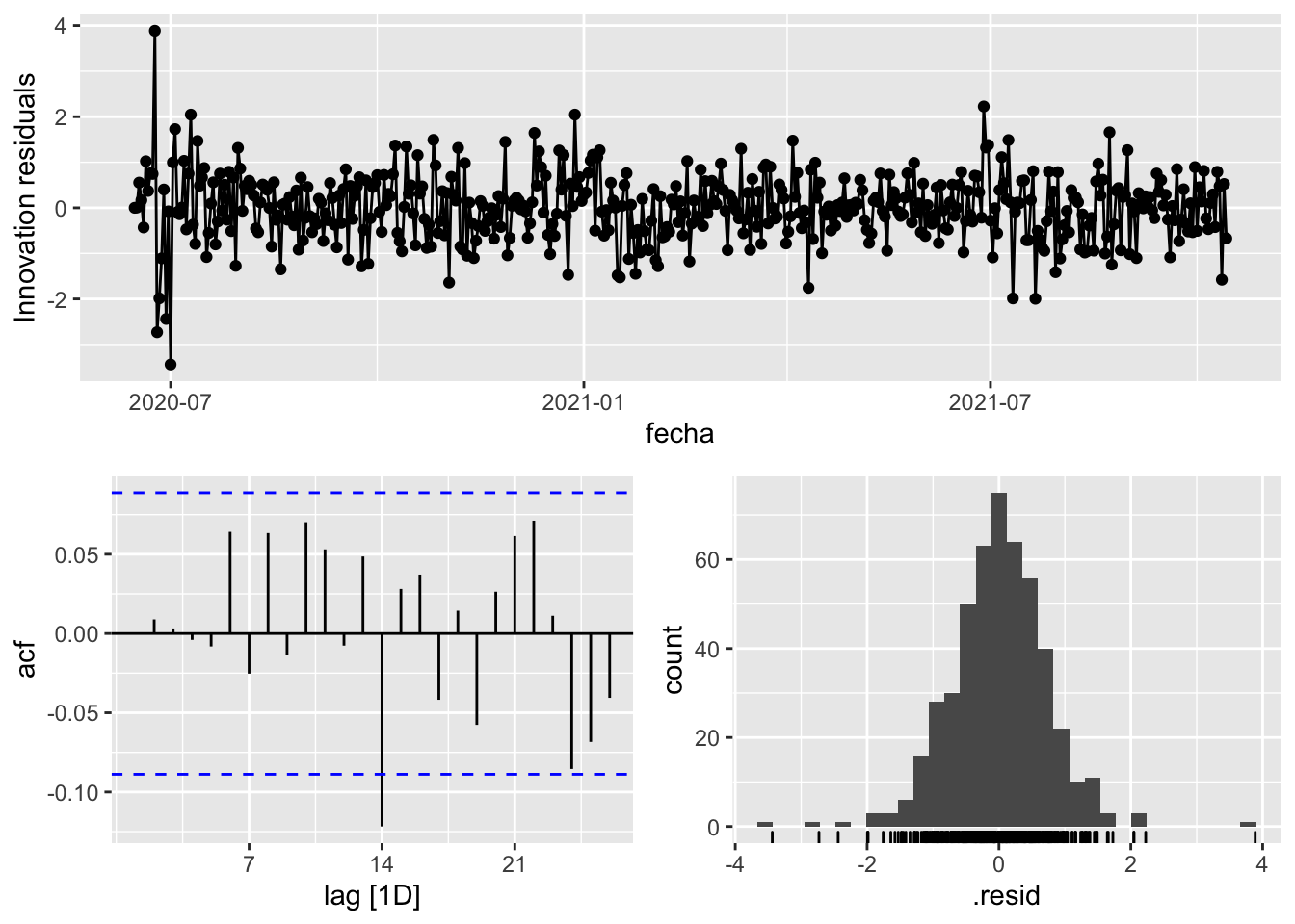
augment(fit_model) %>%
      features(.innov, ljung_box, lag=7)
# A tibble: 3 × 4
provincia .model lb_stat lb_pvalue
<chr> <chr> <dbl> <dbl>
1 Málaga arima_at1 6.37 0.497
2 Málaga arima_at2 2.44 0.932
3 Málaga Snaive 1361. 0 augment(fit_model) %>%
features(.innov, ljung_box, lag=14)# A tibble: 3 × 4
provincia .model lb_stat lb_pvalue
<chr> <chr> <dbl> <dbl>
1 Málaga arima_at1 20.2 0.125
2 Málaga arima_at2 17.1 0.252
3 Málaga Snaive 1956. 0 augment(fit_model) %>%
features(.innov, ljung_box, lag=21)# A tibble: 3 × 4
provincia .model lb_stat lb_pvalue
<chr> <chr> <dbl> <dbl>
1 Málaga arima_at1 26.7 0.179
2 Málaga arima_at2 23.1 0.336
3 Málaga Snaive 2100. 0 augment(fit_model) %>%
features(.innov, ljung_box, lag=90)# A tibble: 3 × 4
provincia .model lb_stat lb_pvalue
<chr> <chr> <dbl> <dbl>
1 Málaga arima_at1 131. 0.00301
2 Málaga arima_at2 119. 0.0227
3 Málaga Snaive 3195. 0 # To predict future values of infections, we need to pass the model future/prediction values of the complementary variables tmed and mobility
# We are going to select those from the test dataset
data_fc_h7 <- data_Malaga_test %>%
select(-num_casos) %>%
slice(1:7)
data_fc_h14 <- data_Malaga_test %>%
select(-num_casos) %>%
slice(1:14)
data_fc_h21 <- data_Malaga_test %>%
select(-num_casos) %>%
slice(1:21)
data_fc_h90 <- data_Malaga_test %>%
select(-num_casos) %>%
slice(1:90)# Significant spikes out of 30 is still consistent with white noise
# To be sure, use a Ljung-Box test, which has a large p-value, confirming that
# the residuals are similar to white noise.
# Note that the alternative models also passed this test.
#
# Forecast
fc_h7 <- fabletools::forecast(fit_model, new_data = data_fc_h7)
fc_h14 <- fabletools::forecast(fit_model, new_data = data_fc_h14)
fc_h21 <- fabletools::forecast(fit_model, new_data = data_fc_h21)
fc_h90 <- fabletools::forecast(fit_model, new_data = data_fc_h90)7 days
# Plots
fc_h7 %>%
      autoplot(
            data_Malaga_test %>%
                  filter(fecha <= as.Date("2021-10-14", format = "%Y-%m-%d")+days(9))
      ) +
      labs(y = "Nº cases", title = "Malaga - forecast h7")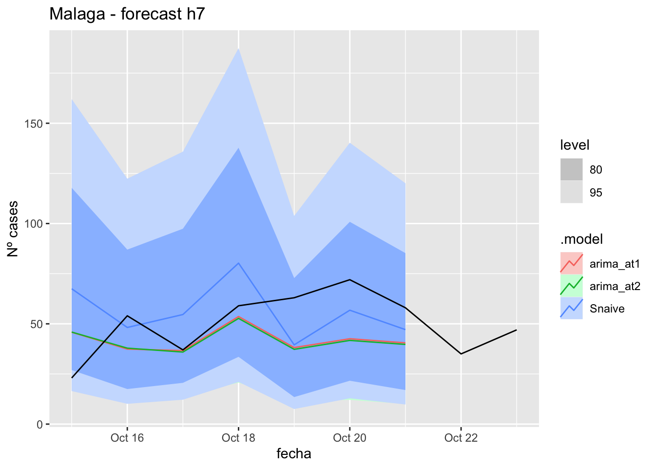
fc_h7 %>%
      autoplot(
            data_Malaga %>%
                  filter(fecha <= as.Date("2021-10-14", format = "%Y-%m-%d")+days(9) &
                               fecha > as.Date("2021-07-01", format = "%Y-%m-%d"))
      ) +
      labs(y = "Nº cases", title = "Malaga - forecast h7")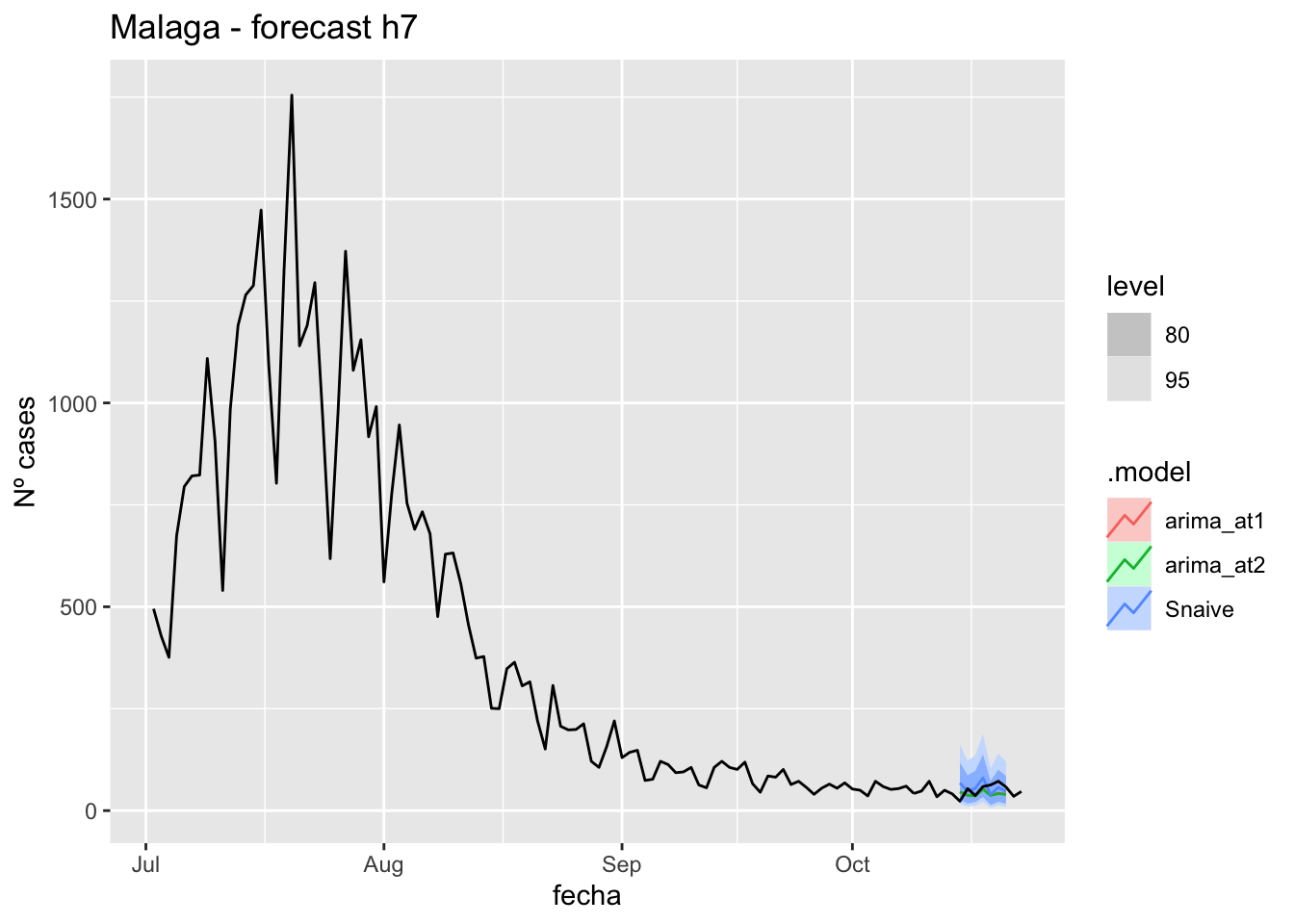
# Accuracy
fabletools::accuracy(fc_h7, data_Malaga)
# A tibble: 3 × 11
.model provincia .type ME RMSE MAE MPE MAPE MASE RMSSE ACF1
<chr> <chr> <chr> <dbl> <dbl> <dbl> <dbl> <dbl> <dbl> <dbl> <dbl>
1 arima_at1 Málaga Test 10.2 19.3 16.7 7.44 35.8 0.170 0.114 0.0661
2 arima_at2 Málaga Test 10.7 19.8 17.2 8.32 36.8 0.175 0.117 0.0950
3 Snaive Málaga Test -4.00 22.9 19.8 -27.0 52.2 0.201 0.135 0.012314 days
# Plots
fc_h14 %>%
      autoplot(
            data_Malaga_test %>%
                  filter(fecha <= as.Date("2021-10-14", format = "%Y-%m-%d")+days(16))
      ) +
      labs(y = "Nº cases", title = "Malaga - forecast h14")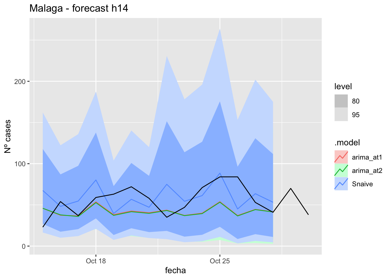
fc_h14 %>%
      autoplot(
            data_Malaga %>%
                  filter(fecha <= as.Date("2021-10-14", format = "%Y-%m-%d")+days(16) &
                               fecha > as.Date("2021-07-01", format = "%Y-%m-%d"))
      ) +
      labs(y = "Nº cases", title = "Malaga - forecast h14")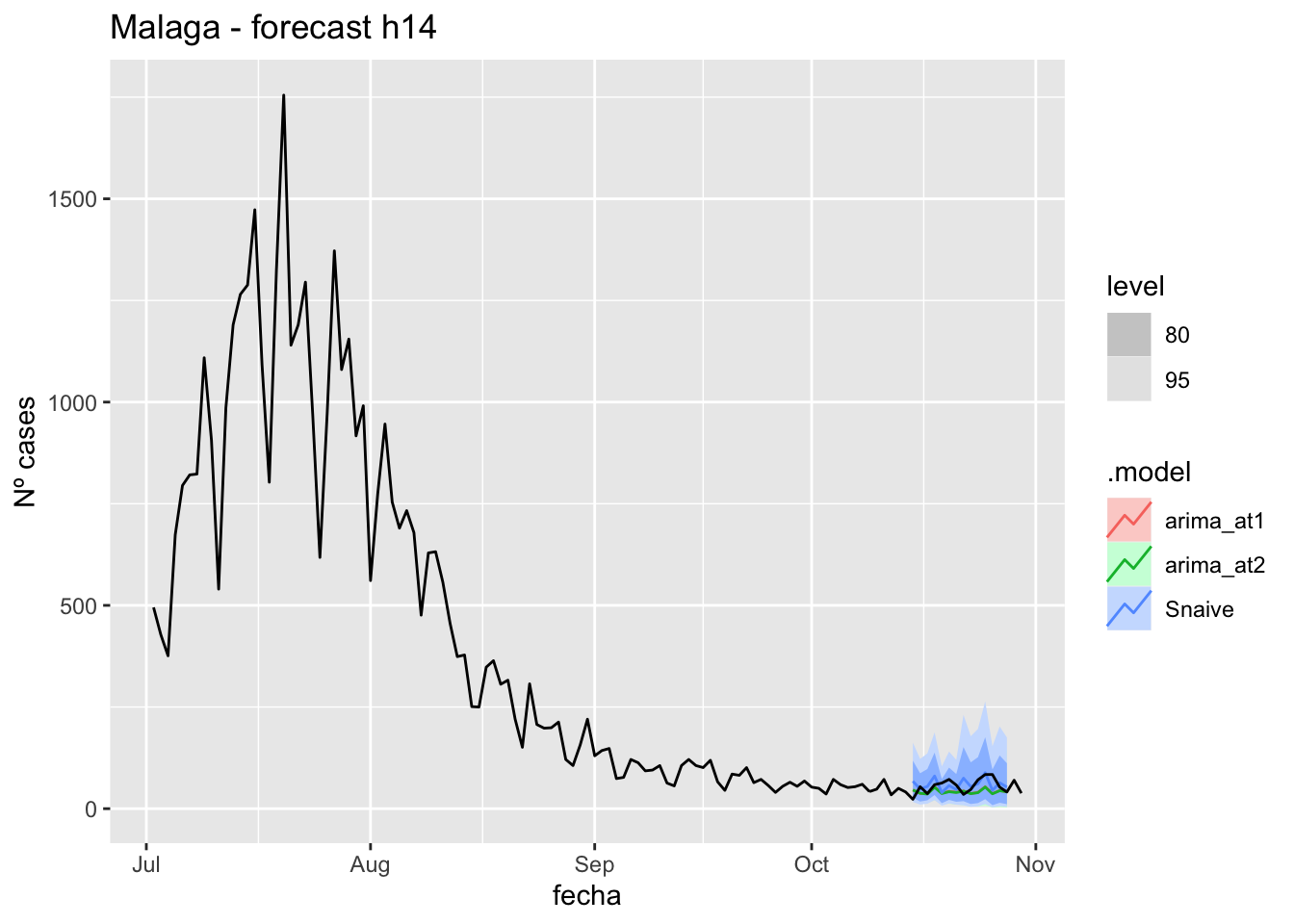
# Accuracy
fabletools::accuracy(fc_h14, data_Malaga)
# A tibble: 3 × 11
.model provincia .type ME RMSE MAE MPE MAPE MASE RMSSE ACF1
<chr> <chr> <chr> <dbl> <dbl> <dbl> <dbl> <dbl> <dbl> <dbl> <dbl>
1 arima_at1 Málaga Test 13.4 22.2 18.0 14.1 32.1 0.183 0.131 0.179
2 arima_at2 Málaga Test 13.9 22.6 18.4 14.9 32.7 0.187 0.134 0.190
3 Snaive Málaga Test -3.86 22.7 18.7 -22.4 43.6 0.190 0.134 -0.097321 days
# Plots
fc_h21 %>%
      autoplot(
            data_Malaga_test %>%
                  filter(fecha <= as.Date("2021-10-14", format = "%Y-%m-%d")+days(23))
      ) +
      labs(y = "Nº cases", title = "Malaga - forecast h21")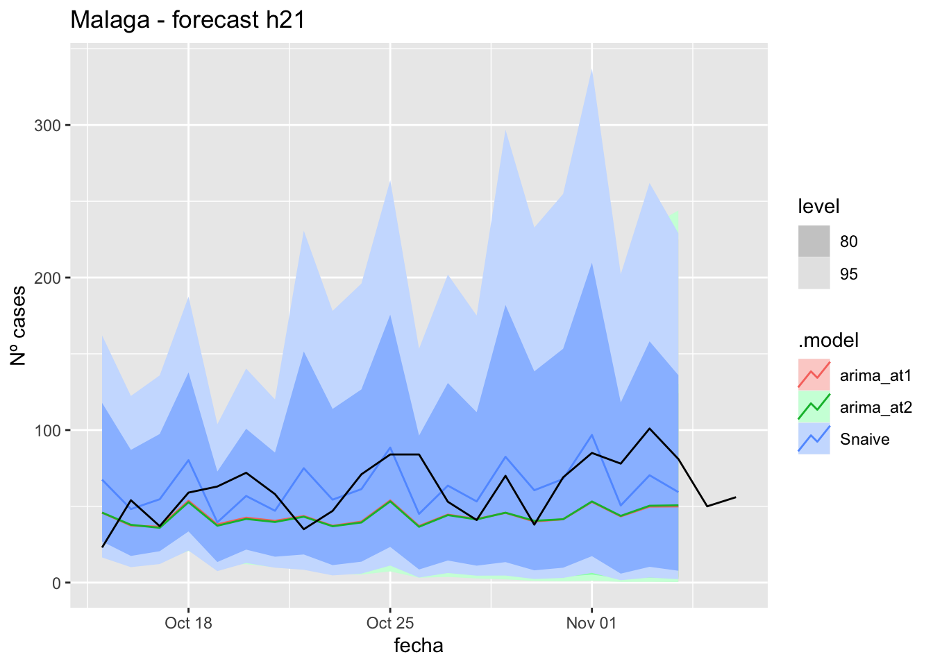
fc_h21 %>%
      autoplot(
            data_Malaga %>%
                  filter(fecha <= as.Date("2021-10-14", format = "%Y-%m-%d")+days(23) &
                               fecha > as.Date("2021-07-01", format = "%Y-%m-%d"))
      ) +
      labs(y = "Nº cases", title = "Malaga - forecast h21")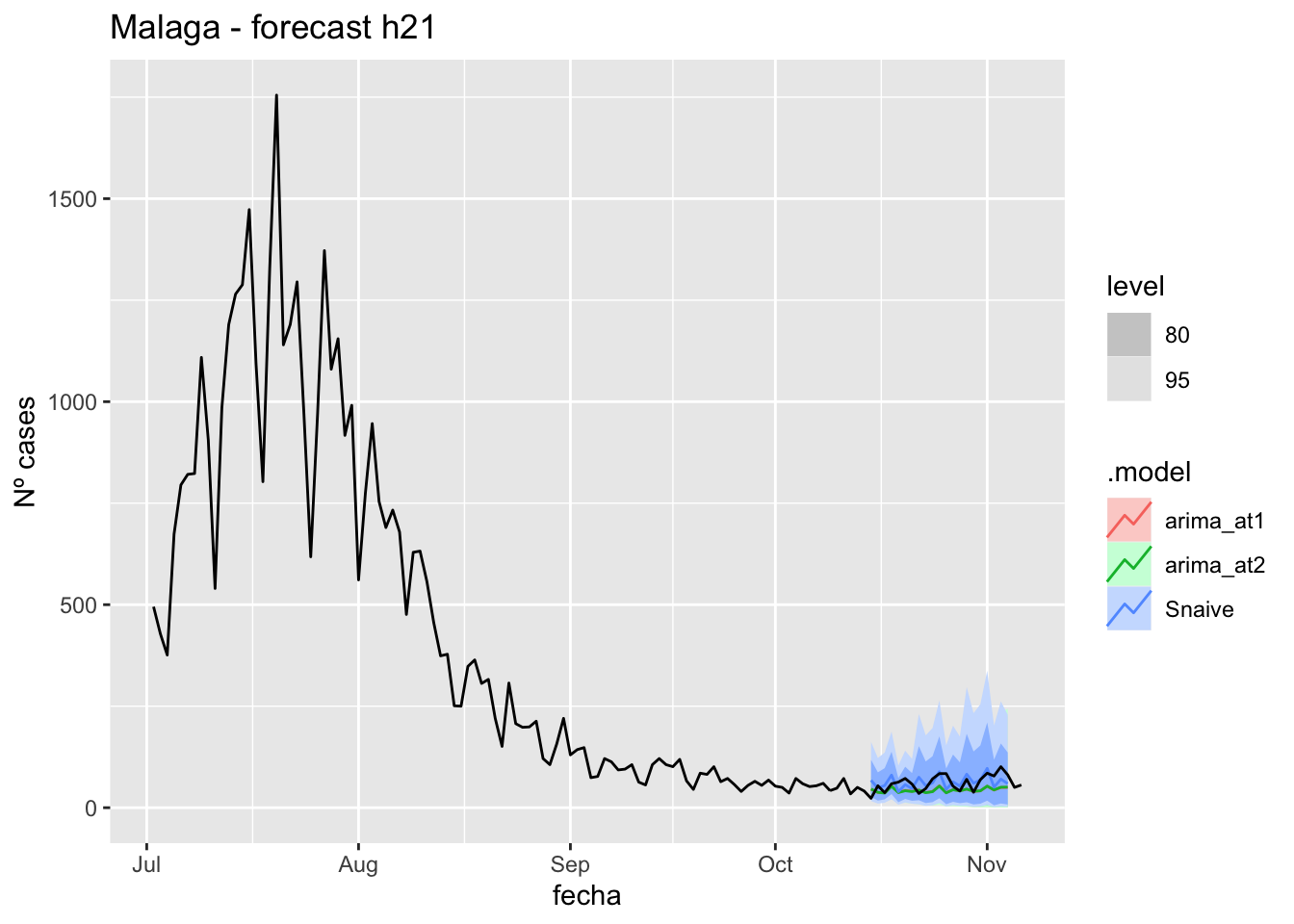
# Accuracy
fabletools::accuracy(fc_h21, data_Malaga)
# A tibble: 3 × 11
.model provincia .type ME RMSE MAE MPE MAPE MASE RMSSE ACF1
<chr> <chr> <chr> <dbl> <dbl> <dbl> <dbl> <dbl> <dbl> <dbl> <dbl>
1 arima_at1 Málaga Test 18.4 25.9 21.7 20.9 33.3 0.220 0.153 0.249
2 arima_at2 Málaga Test 18.6 26.0 21.9 21.2 33.7 0.222 0.154 0.244
3 Snaive Málaga Test -0.951 22.0 18.6 -14.8 37.9 0.188 0.130 0.088690 days
# Plots
fc_h90 %>%
      autoplot(
            data_Malaga_test %>%
                  filter(fecha <= as.Date("2021-10-14", format = "%Y-%m-%d")+days(92))
      ) +
      labs(y = "Nº cases", title = "Malaga - forecast h90")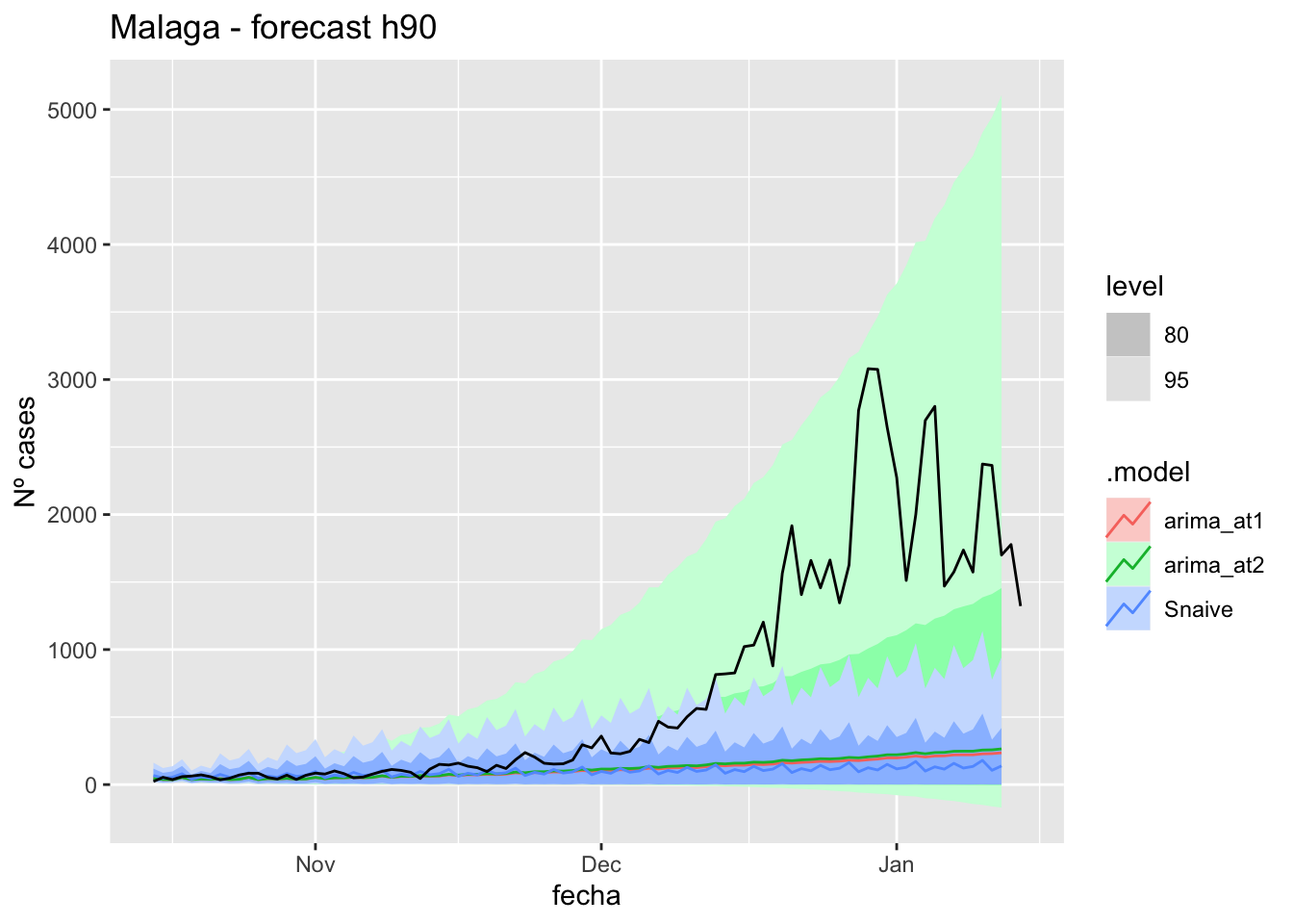
fc_h90 %>%
      autoplot(
            data_Malaga %>%
                  filter(fecha <= as.Date("2021-10-14", format = "%Y-%m-%d")+days(92) &
                               fecha > as.Date("2021-07-01", format = "%Y-%m-%d"))
      ) +
      labs(y = "Nº cases", title = "Malaga - forecast h90")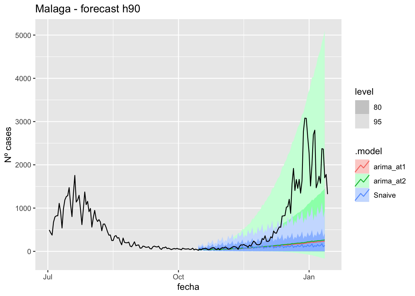
# Accuracy
fabletools::accuracy(fc_h90, data_Malaga)
# A tibble: 3 × 11
.model provincia .type ME RMSE MAE MPE MAPE MASE RMSSE ACF1
<chr> <chr> <chr> <dbl> <dbl> <dbl> <dbl> <dbl> <dbl> <dbl> <dbl>
1 arima_at1 Málaga Test 606. 1013. 607. 55.8 59.8 6.17 5.99 0.927
2 arima_at2 Málaga Test 596. 1001. 597. 54.1 58.3 6.07 5.91 0.926
3 Snaive Málaga Test 620. 1049. 628. 44.9 62.3 6.37 6.20 0.929Sevilla
data_Sevilla <- covid_data %>%
      filter(provincia == "Sevilla") %>%
      filter(fecha > as.Date("2020-06-14", format = "%Y-%m-%d")) %>%
      select(provincia, fecha, num_casos, tmed) %>%
      drop_na() %>%
      as_tsibble(key = provincia, index = fecha)
data_Sevilla
# A tsibble: 653 x 4 [1D]
# Key: provincia [1]
provincia fecha num_casos tmed
<chr> <date> <dbl> <dbl>
1 Sevilla 2020-06-15 2 23.1
2 Sevilla 2020-06-16 1 24.0
3 Sevilla 2020-06-17 0 24.9
4 Sevilla 2020-06-18 0 25.8
5 Sevilla 2020-06-19 0 26.6
6 Sevilla 2020-06-20 0 27.5
7 Sevilla 2020-06-21 0 28.4
8 Sevilla 2020-06-22 1 29.3
9 Sevilla 2020-06-23 0 30.2
10 Sevilla 2020-06-24 1 29.4
# … with 643 more rowsdata_Sevilla_train <- data_Sevilla %>%
filter(fecha <= as.Date("2021-10-14", format = "%Y-%m-%d"))
summary(data_Sevilla_train$fecha) Min. 1st Qu. Median Mean 3rd Qu. Max.
"2020-06-15" "2020-10-14" "2021-02-13" "2021-02-13" "2021-06-14" "2021-10-14" data_Sevilla_test <- data_Sevilla %>%
filter(fecha > as.Date("2021-10-14", format = "%Y-%m-%d"))
summary(data_Sevilla_test$fecha) Min. 1st Qu. Median Mean 3rd Qu. Max.
"2021-10-15" "2021-11-25" "2022-01-05" "2022-01-05" "2022-02-15" "2022-03-29" # Lamba for num_casos
lambda_Sevilla_casos <- data_Sevilla %>%
features(num_casos, features = guerrero) %>%
pull(lambda_guerrero)
lambda_Sevilla_casos[1] 0.1933674# Lamba for average temp
lambda_Sevilla_tmed <- data_Sevilla %>%
features(tmed, features = guerrero) %>%
pull(lambda_guerrero)
lambda_Sevilla_tmed[1] 0.9333023fit_model <- data_Sevilla_train %>%
model(
arima_at1 = ARIMA(box_cox(num_casos, lambda_Sevilla_casos) ~
box_cox(tmed, lambda_Sevilla_tmed)),
arima_at2 = ARIMA(box_cox(num_casos, lambda_Sevilla_casos) ~
box_cox(tmed, lambda_Sevilla_tmed),
stepwise = FALSE, approx = FALSE),
Snaive = SNAIVE(box_cox(num_casos, lambda_Sevilla_casos))
)
# Show and report model
fit_model# A mable: 1 x 4
# Key: provincia [1]
provincia arima_at1
<chr> <model>
1 Sevilla <LM w/ ARIMA(3,1,1)(2,0,0)[7] errors>
# … with 2 more variables: arima_at2 <model>, Snaive <model>glance(fit_model)# A tibble: 3 × 9
provincia .model sigma2 log_lik AIC AICc BIC ar_roots ma_roots
<chr> <chr> <dbl> <dbl> <dbl> <dbl> <dbl> <list> <list>
1 Sevilla arima_at1 0.924 -669. 1355. 1355. 1388. <cpl [17]> <cpl [1]>
2 Sevilla arima_at2 0.922 -669. 1354. 1354. 1387. <cpl [18]> <cpl [0]>
3 Sevilla Snaive 2.02 NA NA NA NA <NULL> <NULL> fit_model %>%
pivot_longer(-provincia,
names_to = ".model",
values_to = "orders") %>%
left_join(glance(fit_model), by = c("provincia", ".model")) %>%
arrange(AICc) %>%
select(.model:BIC)# A mable: 3 x 7
# Key: .model [3]
.model orders sigma2 log_lik AIC AICc BIC
<chr> <model> <dbl> <dbl> <dbl> <dbl> <dbl>
1 arima_… <LM w/ ARIMA(4,1,0)(2,0,0)[7] errors> 0.922 -669. 1354. 1354. 1387.
2 arima_… <LM w/ ARIMA(3,1,1)(2,0,0)[7] errors> 0.924 -669. 1355. 1355. 1388.
3 Snaive <SNAIVE> 2.02 NA NA NA NA # We use a Ljung-Box test >> large p-value, confirms residuals are similar / considered to white noise
fit_model %>%
select(Snaive) %>%
gg_tsresiduals()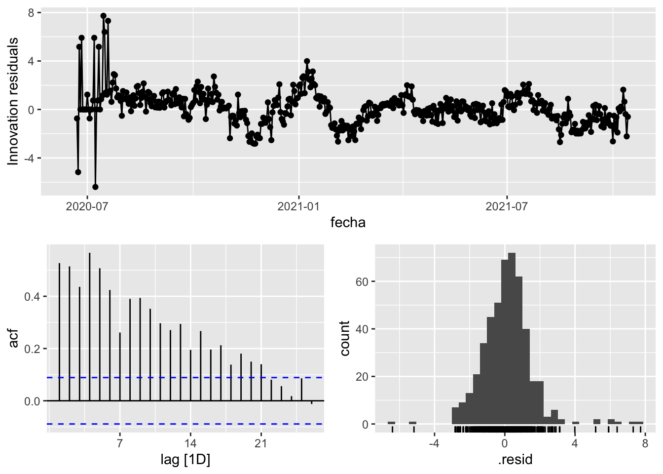
fit_model %>%
      select(arima_at1) %>%
      gg_tsresiduals()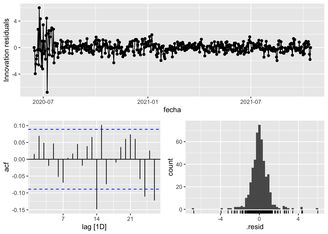
fit_model %>%
      select(arima_at2) %>%
      gg_tsresiduals()
augment(fit_model) %>%
      features(.innov, ljung_box, lag=7)
# A tibble: 3 × 4
provincia .model lb_stat lb_pvalue
<chr> <chr> <dbl> <dbl>
1 Sevilla arima_at1 8.68 0.276
2 Sevilla arima_at2 7.66 0.363
3 Sevilla Snaive 757. 0 augment(fit_model) %>%
features(.innov, ljung_box, lag=14)# A tibble: 3 × 4
provincia .model lb_stat lb_pvalue
<chr> <chr> <dbl> <dbl>
1 Sevilla arima_at1 24.1 0.0446
2 Sevilla arima_at2 23.3 0.0555
3 Sevilla Snaive 1110. 0 augment(fit_model) %>%
features(.innov, ljung_box, lag=21)# A tibble: 3 × 4
provincia .model lb_stat lb_pvalue
<chr> <chr> <dbl> <dbl>
1 Sevilla arima_at1 37.5 0.0147
2 Sevilla arima_at2 36.7 0.0181
3 Sevilla Snaive 1235. 0 augment(fit_model) %>%
features(.innov, ljung_box, lag=90)# A tibble: 3 × 4
provincia .model lb_stat lb_pvalue
<chr> <chr> <dbl> <dbl>
1 Sevilla arima_at1 103. 0.166
2 Sevilla arima_at2 102. 0.182
3 Sevilla Snaive 1692. 0 # To predict future values of infections, we need to pass the model future/prediction values of the complementary variables tmed and mobility
# We are going to select those from the test dataset
data_fc_h7 <- data_Sevilla_test %>%
select(-num_casos) %>%
slice(1:7)
data_fc_h14 <- data_Sevilla_test %>%
select(-num_casos) %>%
slice(1:14)
data_fc_h21 <- data_Sevilla_test %>%
select(-num_casos) %>%
slice(1:21)
data_fc_h90 <- data_Sevilla_test %>%
select(-num_casos) %>%
slice(1:90)# Significant spikes out of 30 is still consistent with white noise
# To be sure, use a Ljung-Box test, which has a large p-value, confirming that
# the residuals are similar to white noise.
# Note that the alternative models also passed this test.
#
# Forecast
fc_h7 <- fabletools::forecast(fit_model, new_data = data_fc_h7)
fc_h14 <- fabletools::forecast(fit_model, new_data = data_fc_h14)
fc_h21 <- fabletools::forecast(fit_model, new_data = data_fc_h21)
fc_h90 <- fabletools::forecast(fit_model, new_data = data_fc_h90)7 days
# Plots
fc_h7 %>%
      autoplot(
            data_Sevilla_test %>%
                  filter(fecha <= as.Date("2021-10-14", format = "%Y-%m-%d")+days(9))
      ) +
      labs(y = "Nº cases", title = "Sevilla - forecast h7")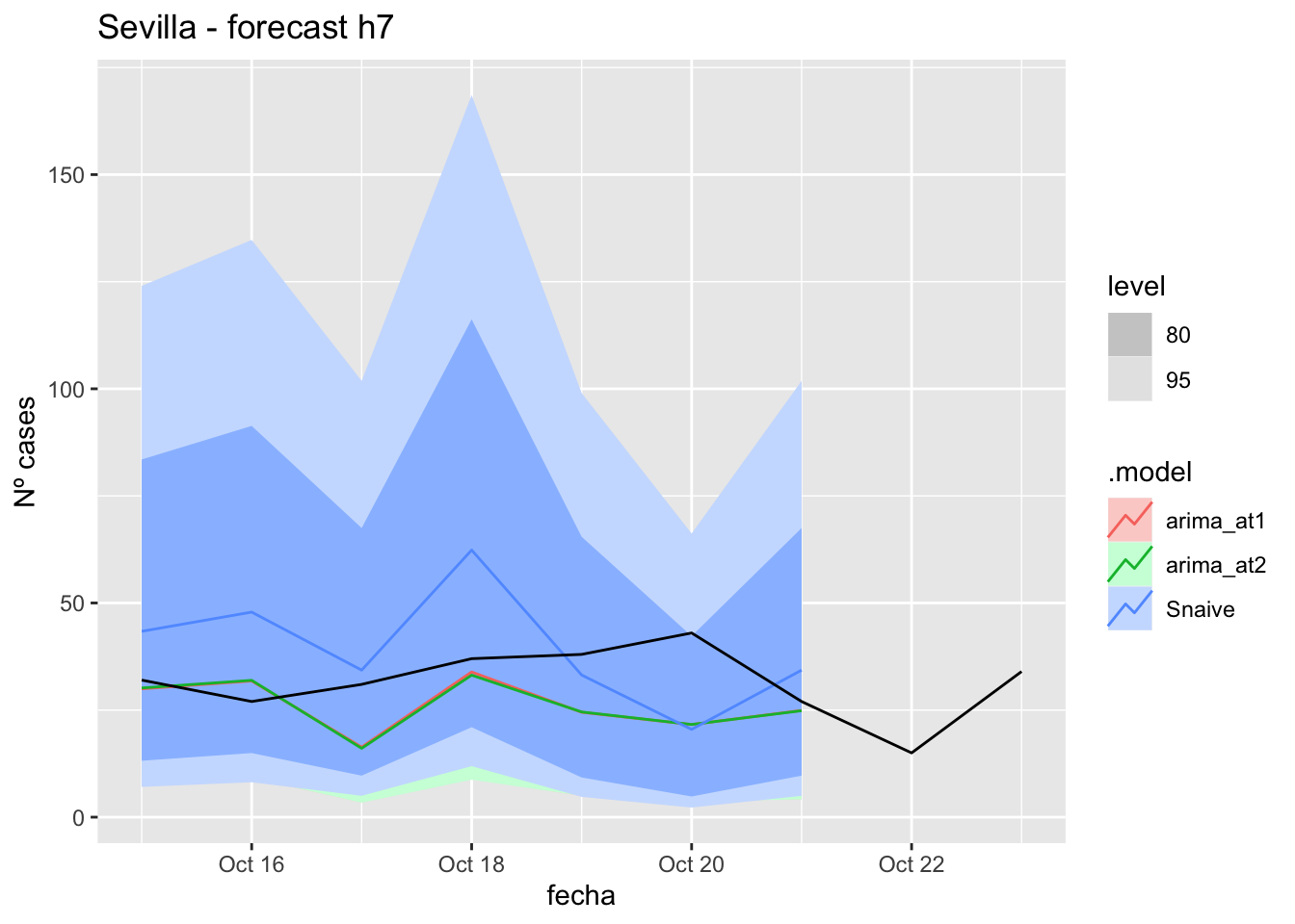
fc_h7 %>%
      autoplot(
            data_Sevilla %>%
                  filter(fecha <= as.Date("2021-10-14", format = "%Y-%m-%d")+days(9) &
                               fecha > as.Date("2021-07-01", format = "%Y-%m-%d"))
      ) +
      labs(y = "Nº cases", title = "Sevilla - forecast h7")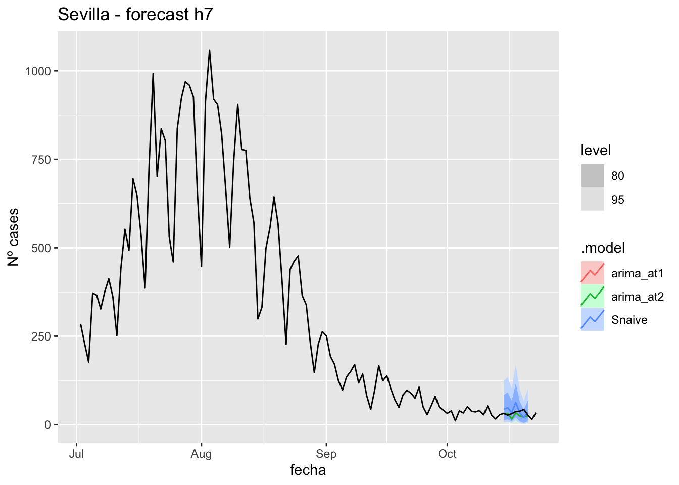
# Accuracy
fabletools::accuracy(fc_h7, data_Sevilla)
# A tibble: 3 × 11
.model provincia .type ME RMSE MAE MPE MAPE MASE RMSSE ACF1
<chr> <chr> <chr> <dbl> <dbl> <dbl> <dbl> <dbl> <dbl> <dbl> <dbl>
1 arima_at1 Sevilla Test 7.42 11.3 8.79 19.6 24.7 0.0869 0.0717 -0.137
2 arima_at2 Sevilla Test 7.51 11.4 8.93 19.8 25.1 0.0882 0.0722 -0.123
3 Snaive Sevilla Test -5.85 16.0 13.7 -22.0 40.6 0.135 0.102 0.031014 days
# Plots
fc_h14 %>%
      autoplot(
            data_Sevilla_test %>%
                  filter(fecha <= as.Date("2021-10-14", format = "%Y-%m-%d")+days(16))
      ) +
      labs(y = "Nº cases", title = "Sevilla - forecast h14")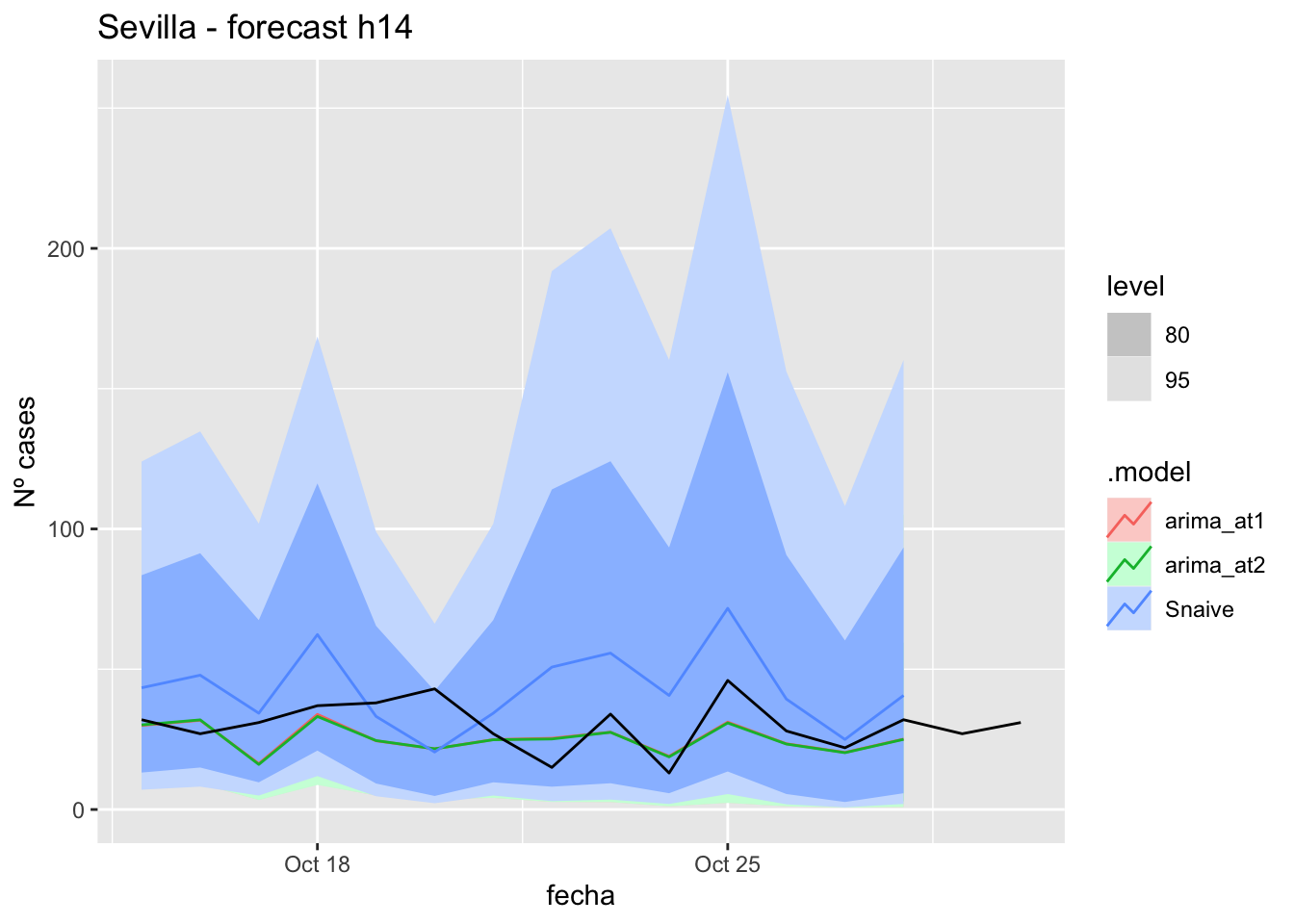
fc_h14 %>%
autoplot(
data_Sevilla %>%
filter(fecha <= as.Date("2021-10-14", format = "%Y-%m-%d")+days(16) &
fecha > as.Date("2021-07-01", format = "%Y-%m-%d"))
) +
labs(y = "Nº cases", title = "Sevilla - forecast h14")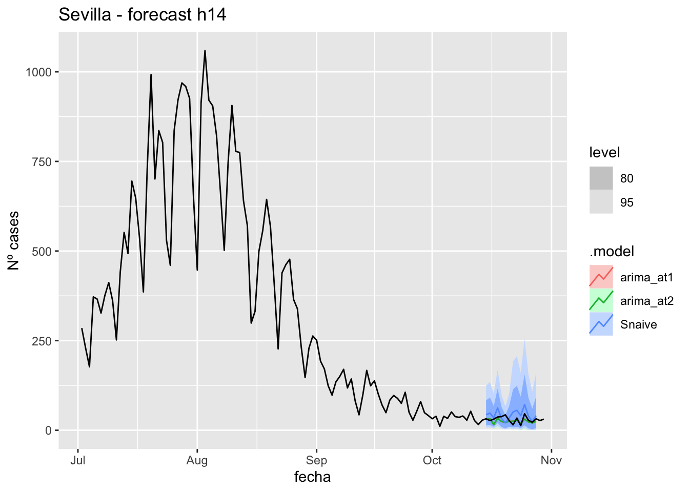
# Accuracy
fabletools::accuracy(fc_h14, data_Sevilla)# A tibble: 3 × 11
.model provincia .type ME RMSE MAE MPE MAPE MASE RMSSE ACF1
<chr> <chr> <chr> <dbl> <dbl> <dbl> <dbl> <dbl> <dbl> <dbl> <dbl>
1 arima_at1 Sevilla Test 5.00 9.90 8.02 8.47 27.5 0.0793 0.0628 -0.116
2 arima_at2 Sevilla Test 5.13 9.96 8.10 8.97 27.6 0.0801 0.0631 -0.108
3 Snaive Sevilla Test -12.5 19.3 16.4 -57.6 66.9 0.162 0.122 0.27521 days
# Plots
fc_h21 %>%
autoplot(
data_Sevilla_test %>%
filter(fecha <= as.Date("2021-10-14", format = "%Y-%m-%d")+days(23))
) +
labs(y = "Nº cases", title = "Sevilla - forecast h21")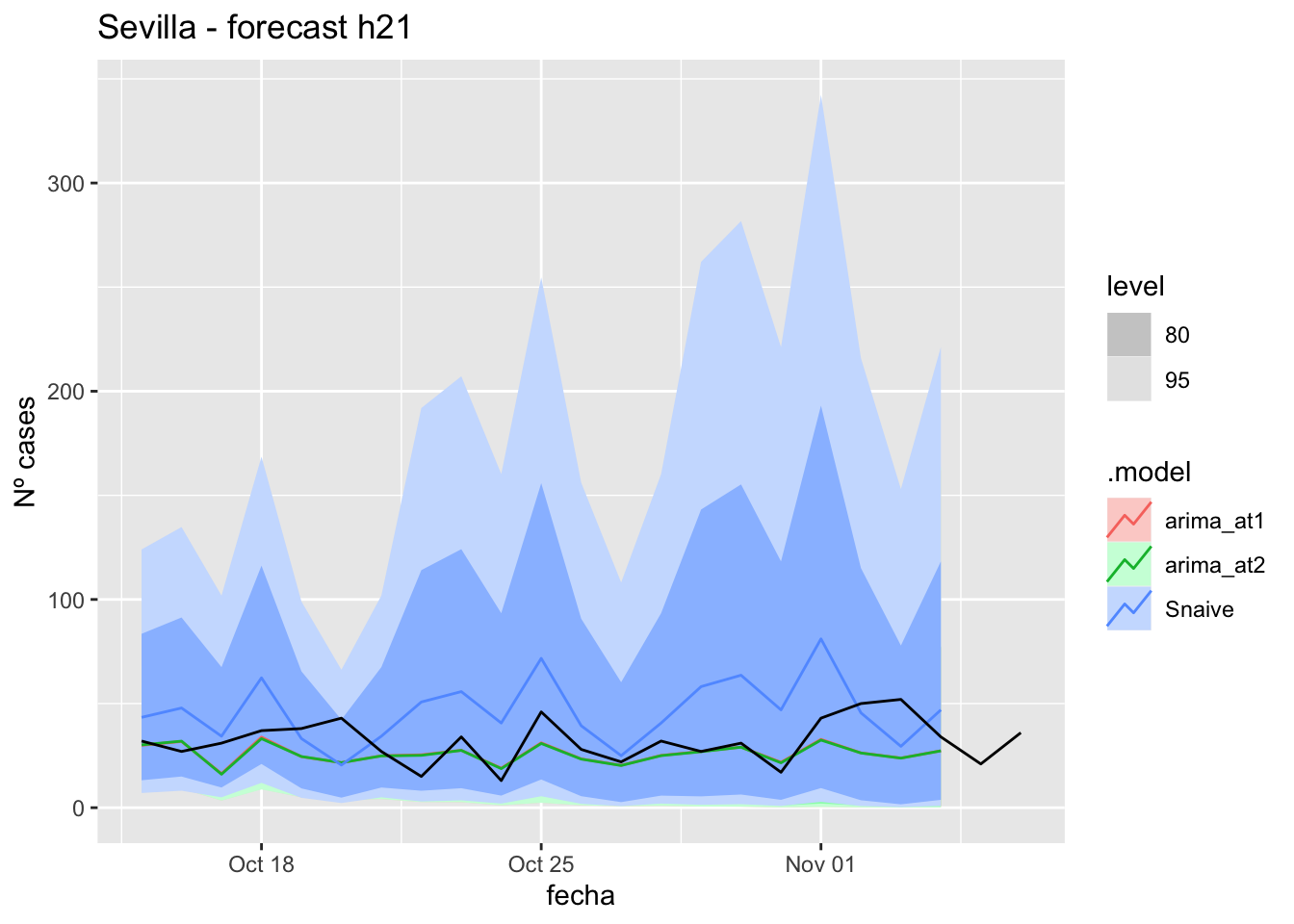
fc_h21 %>%
autoplot(
data_Sevilla %>%
filter(fecha <= as.Date("2021-10-14", format = "%Y-%m-%d")+days(23) &
fecha > as.Date("2021-07-01", format = "%Y-%m-%d"))
) +
labs(y = "Nº cases", title = "Sevilla - forecast h21")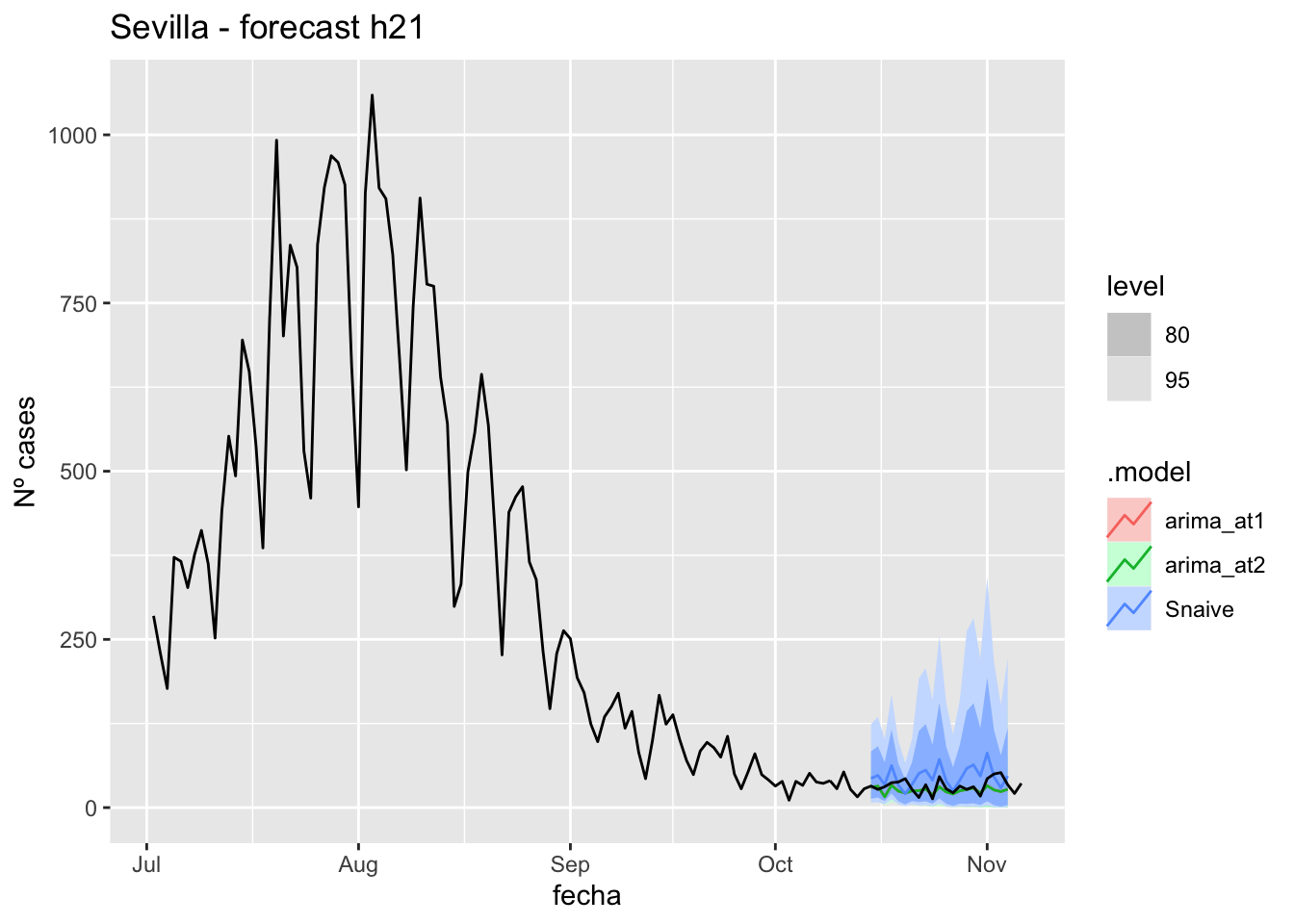
# Accuracy
fabletools::accuracy(fc_h21, data_Sevilla)# A tibble: 3 × 11
.model provincia .type ME RMSE MAE MPE MAPE MASE RMSSE ACF1
<chr> <chr> <chr> <dbl> <dbl> <dbl> <dbl> <dbl> <dbl> <dbl> <dbl>
1 arima_at1 Sevilla Test 6.47 11.8 8.94 11.5 26.9 0.0883 0.0745 0.191
2 arima_at2 Sevilla Test 6.59 11.8 9.01 12.0 26.9 0.0890 0.0749 0.194
3 Snaive Sevilla Test -13.9 22.1 19.1 -60.8 72.0 0.189 0.140 0.32790 days
# Plots
fc_h90 %>%
autoplot(
data_Sevilla_test %>%
filter(fecha <= as.Date("2021-10-14", format = "%Y-%m-%d")+days(92))
) +
labs(y = "Nº cases", title = "Sevilla - forecast h90")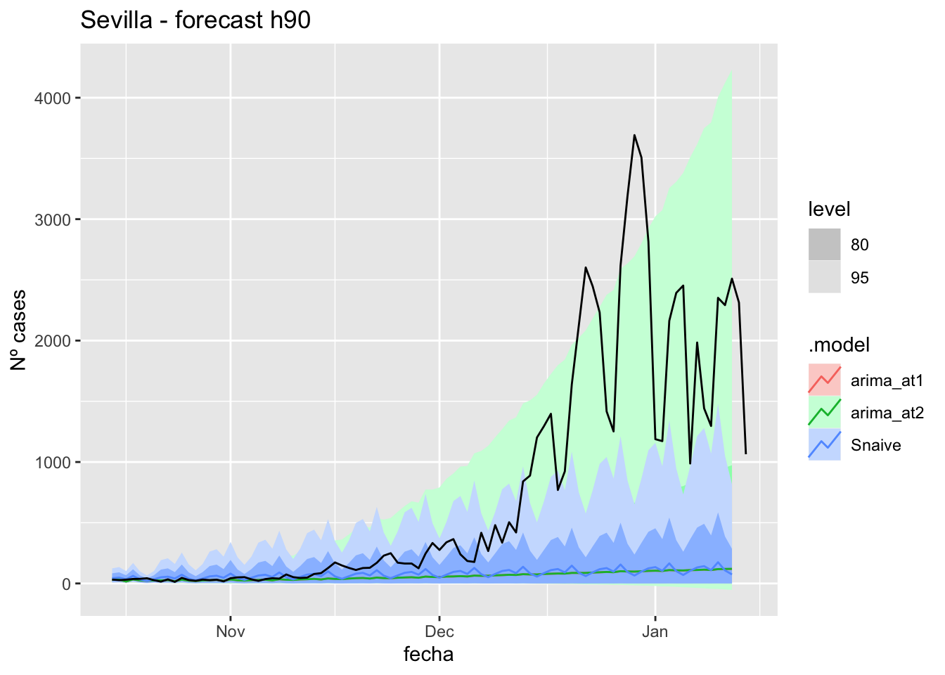
fc_h90 %>%
autoplot(
data_Sevilla %>%
filter(fecha <= as.Date("2021-10-14", format = "%Y-%m-%d")+days(92) &
fecha > as.Date("2021-07-01", format = "%Y-%m-%d"))
) +
labs(y = "Nº cases", title = "Sevilla - forecast h90")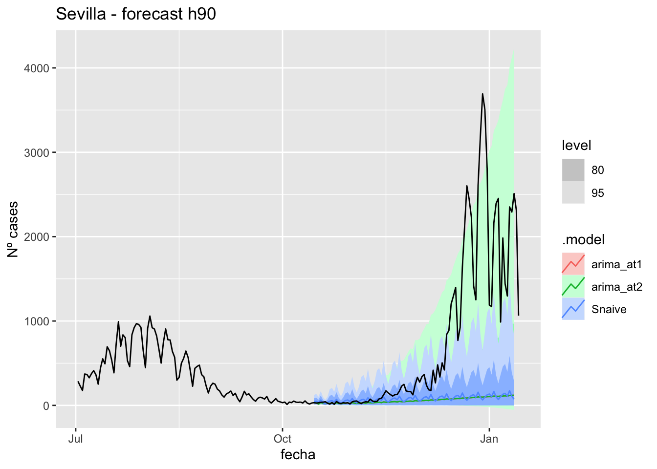
# Accuracy
fabletools::accuracy(fc_h90, data_Sevilla)# A tibble: 3 × 11
.model provincia .type ME RMSE MAE MPE MAPE MASE RMSSE ACF1
<chr> <chr> <chr> <dbl> <dbl> <dbl> <dbl> <dbl> <dbl> <dbl> <dbl>
1 arima_at1 Sevilla Test 686. 1166. 687. 61.8 66.2 6.79 7.39 0.892
2 arima_at2 Sevilla Test 686. 1165. 687. 61.9 66.2 6.78 7.39 0.892
3 Snaive Sevilla Test 665. 1161. 677. 31.7 74.6 6.69 7.36 0.892Middel of sixth epidemiological period
Asturias
data_asturias <- covid_data %>%
filter(provincia == "Asturias") %>%
filter(fecha > as.Date("2020-06-14", format = "%Y-%m-%d")) %>%
select(provincia, fecha, num_casos, tmed) %>%
drop_na() %>%
as_tsibble(key = provincia, index = fecha)
data_asturias# A tsibble: 653 x 4 [1D]
# Key: provincia [1]
provincia fecha num_casos tmed
<chr> <date> <dbl> <dbl>
1 Asturias 2020-06-15 0 16
2 Asturias 2020-06-16 1 15.6
3 Asturias 2020-06-17 0 15.6
4 Asturias 2020-06-18 0 15.1
5 Asturias 2020-06-19 0 14.8
6 Asturias 2020-06-20 0 16.8
7 Asturias 2020-06-21 0 18.2
8 Asturias 2020-06-22 0 18.2
9 Asturias 2020-06-23 0 20
10 Asturias 2020-06-24 0 18.2
# … with 643 more rowsdata_asturias_train <- data_asturias %>%
filter(fecha <= as.Date("2022-01-31", format = "%Y-%m-%d"))
summary(data_asturias_train$fecha) Min. 1st Qu. Median Mean 3rd Qu. Max.
"2020-06-15" "2020-11-10" "2021-04-08" "2021-04-08" "2021-09-04" "2022-01-31" data_asturias_test <- data_asturias %>%
filter(fecha > as.Date("2022-01-31", format = "%Y-%m-%d"))
summary(data_asturias_test$fecha) Min. 1st Qu. Median Mean 3rd Qu. Max.
"2022-02-01" "2022-02-15" "2022-03-01" "2022-03-01" "2022-03-15" "2022-03-29" # Lamba for num_casos
lambda_asturias_casos <- data_asturias %>%
features(num_casos, features = guerrero) %>%
pull(lambda_guerrero)
lambda_asturias_casos[1] 0.2278229# Lamba for average temp
lambda_asturias_tmed <- data_asturias %>%
features(tmed, features = guerrero) %>%
pull(lambda_guerrero)
lambda_asturias_tmed[1] 1.056074fit_model <- data_asturias_train %>%
model(
arima_at1 = ARIMA(box_cox(num_casos, lambda_asturias_casos) ~
box_cox(tmed, lambda_asturias_tmed)),
arima_at2 = ARIMA(box_cox(num_casos, lambda_asturias_casos) ~
box_cox(tmed, lambda_asturias_tmed),
stepwise = FALSE, approx = FALSE),
Snaive = SNAIVE(box_cox(num_casos, lambda_asturias_casos))
)
# Show and report model
fit_model# A mable: 1 x 4
# Key: provincia [1]
provincia arima_at1
<chr> <model>
1 Asturias <LM w/ ARIMA(3,1,1)(2,0,0)[7] errors>
# … with 2 more variables: arima_at2 <model>, Snaive <model>glance(fit_model)# A tibble: 3 × 9
provincia .model sigma2 log_lik AIC AICc BIC ar_roots ma_roots
<chr> <chr> <dbl> <dbl> <dbl> <dbl> <dbl> <list> <list>
1 Asturias arima_at1 0.917 -816. 1648. 1648. 1683. <cpl [17]> <cpl [1]>
2 Asturias arima_at2 0.895 -810. 1631. 1631. 1653. <cpl [7]> <cpl [8]>
3 Asturias Snaive 2.53 NA NA NA NA <NULL> <NULL> fit_model %>%
pivot_longer(-provincia,
names_to = ".model",
values_to = "orders") %>%
left_join(glance(fit_model), by = c("provincia", ".model")) %>%
arrange(AICc) %>%
select(.model:BIC)# A mable: 3 x 7
# Key: .model [3]
.model orders sigma2 log_lik AIC AICc BIC
<chr> <model> <dbl> <dbl> <dbl> <dbl> <dbl>
1 arima_… <LM w/ ARIMA(0,1,1)(1,0,1)[7] errors> 0.895 -810. 1631. 1631. 1653.
2 arima_… <LM w/ ARIMA(3,1,1)(2,0,0)[7] errors> 0.917 -816. 1648. 1648. 1683.
3 Snaive <SNAIVE> 2.53 NA NA NA NA # We use a Ljung-Box test >> large p-value, confirms residuals are similar / considered to white noise
fit_model %>%
select(Snaive) %>%
gg_tsresiduals()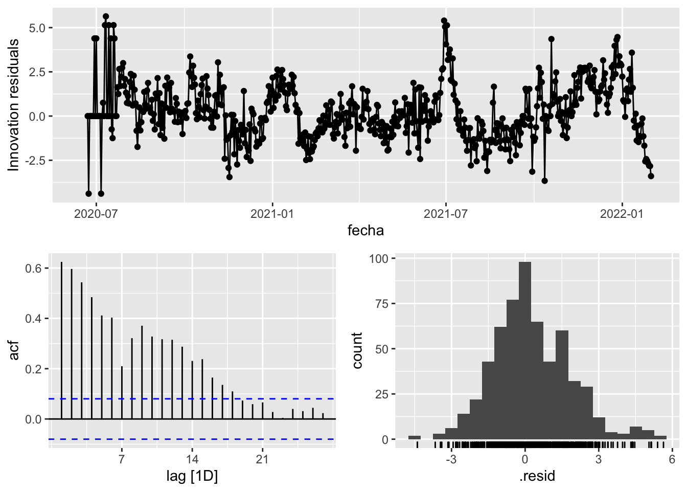
fit_model %>%
select(arima_at1) %>%
gg_tsresiduals()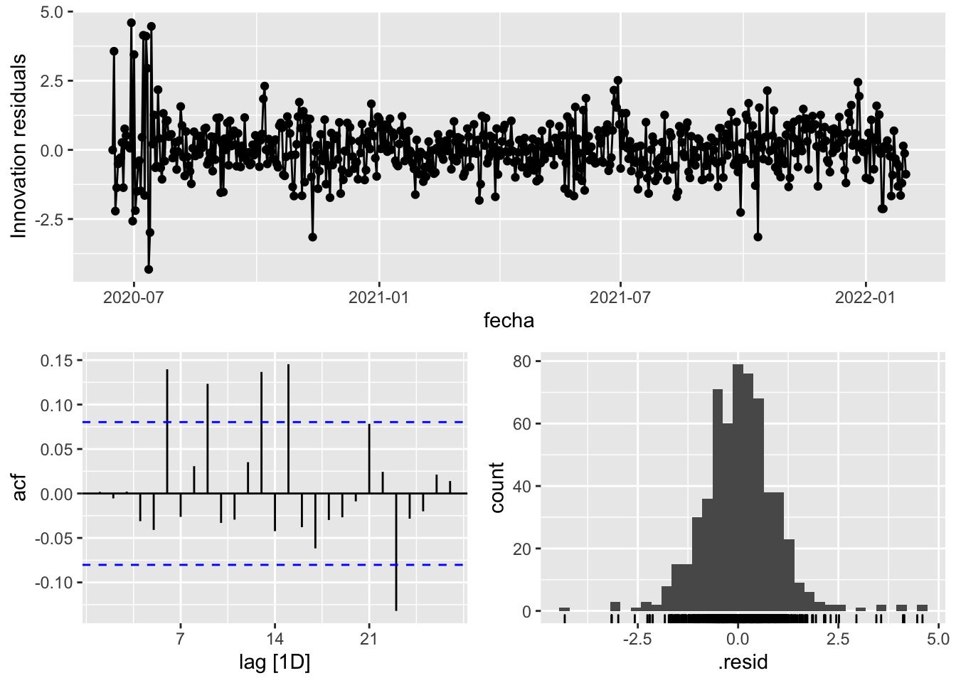
fit_model %>%
select(arima_at2) %>%
gg_tsresiduals()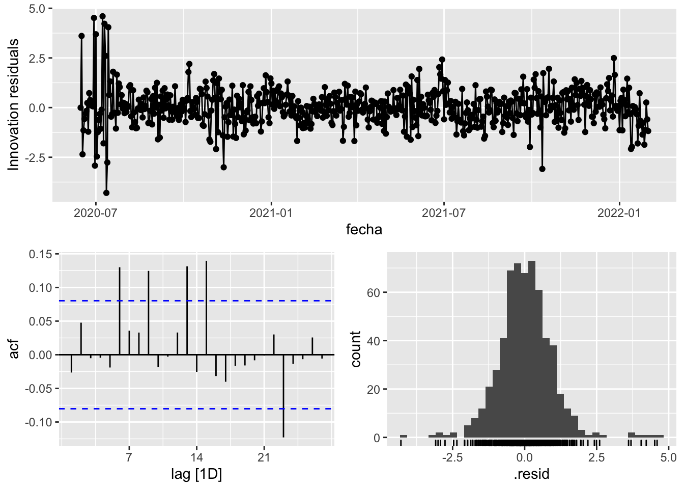
augment(fit_model) %>%
features(.innov, ljung_box, lag=7)# A tibble: 3 × 4
provincia .model lb_stat lb_pvalue
<chr> <chr> <dbl> <dbl>
1 Asturias arima_at1 13.8 0.0544
2 Asturias arima_at2 13.0 0.0717
3 Asturias Snaive 981. 0 augment(fit_model) %>%
features(.innov, ljung_box, lag=14)# A tibble: 3 × 4
provincia .model lb_stat lb_pvalue
<chr> <chr> <dbl> <dbl>
1 Asturias arima_at1 38.1 0.000503
2 Asturias arima_at2 34.9 0.00150
3 Asturias Snaive 1393. 0 augment(fit_model) %>%
features(.innov, ljung_box, lag=21)# A tibble: 3 × 4
provincia .model lb_stat lb_pvalue
<chr> <chr> <dbl> <dbl>
1 Asturias arima_at1 59.1 0.0000173
2 Asturias arima_at2 48.9 0.000522
3 Asturias Snaive 1470. 0 augment(fit_model) %>%
features(.innov, ljung_box, lag=57)# A tibble: 3 × 4
provincia .model lb_stat lb_pvalue
<chr> <chr> <dbl> <dbl>
1 Asturias arima_at1 100. 0.000364
2 Asturias arima_at2 78.5 0.0308
3 Asturias Snaive 1527. 0 # To predict future values of infections, we need to pass the model future/prediction values of the complementary variables tmed and mobility
# We are going to select those from the test dataset
data_fc_h7 <- data_asturias_test %>%
select(-num_casos) %>%
slice(1:7)
data_fc_h14 <- data_asturias_test %>%
select(-num_casos) %>%
slice(1:14)
data_fc_h21 <- data_asturias_test %>%
select(-num_casos) %>%
slice(1:21)
data_fc_h57 <- data_asturias_test %>%
select(-num_casos) %>%
slice(1:57)# Significant spikes out of 30 is still consistent with white noise
# To be sure, use a Ljung-Box test, which has a large p-value, confirming that
# the residuals are similar to white noise.
# Note that the alternative models also passed this test.
#
# Forecast
fc_h7 <- fabletools::forecast(fit_model, new_data = data_fc_h7)
fc_h14 <- fabletools::forecast(fit_model, new_data = data_fc_h14)
fc_h21 <- fabletools::forecast(fit_model, new_data = data_fc_h21)
fc_h57 <- fabletools::forecast(fit_model, new_data = data_fc_h57)7 days
# Plots
fc_h7 %>%
autoplot(
data_asturias_test %>%
filter(fecha <= as.Date("2022-01-31", format = "%Y-%m-%d")+days(7))
) +
labs(y = "Nº cases", title = "Asturias - forecast h7")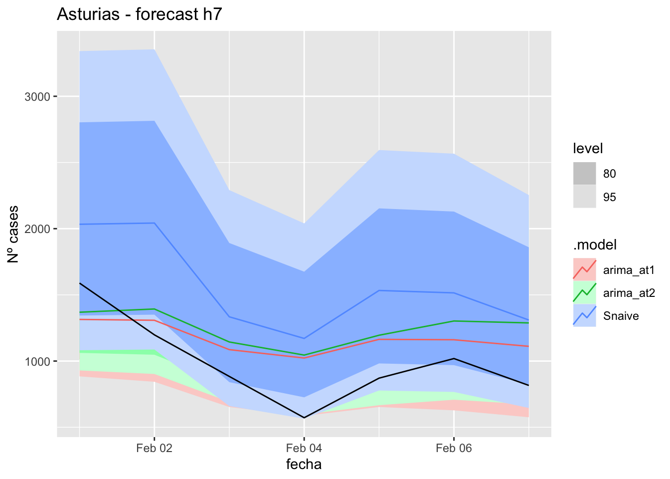
fc_h7 %>%
autoplot(
data_asturias %>%
filter(fecha <= as.Date("2022-01-31", format = "%Y-%m-%d")+days(7) &
fecha > as.Date("2022-01-01", format = "%Y-%m-%d"))
) +
labs(y = "Nº cases", title = "Asturias - forecast h7")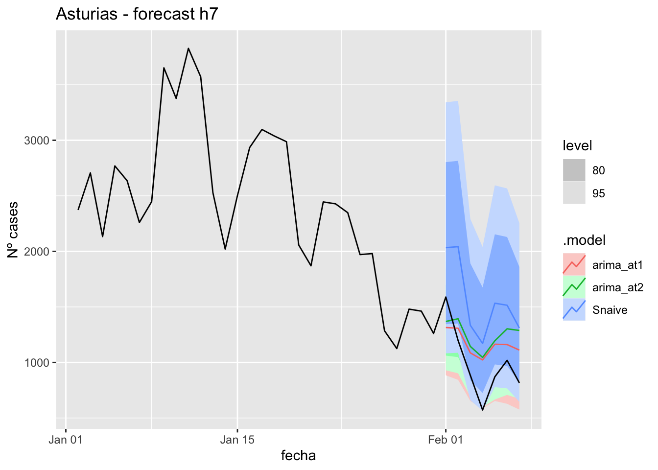
# Accuracy
fabletools::accuracy(fc_h7, data_asturias)# A tibble: 3 × 11
.model provincia .type ME RMSE MAE MPE MAPE MASE RMSSE ACF1
<chr> <chr> <chr> <dbl> <dbl> <dbl> <dbl> <dbl> <dbl> <dbl> <dbl>
1 arima_at1 Asturias Test -174. 274. 253. -25.3 30.3 2.61 1.25 0.192
2 arima_at2 Asturias Test -256. 335. 318. -33.9 37.9 3.29 1.52 0.159
3 Snaive Asturias Test -570. 586. 570. -62.8 62.8 5.89 2.66 -0.55014 days
# Plots
fc_h14 %>%
autoplot(
data_asturias_test %>%
filter(fecha <= as.Date("2022-01-31", format = "%Y-%m-%d")+days(14))
) +
labs(y = "Nº cases", title = "Asturias - forecast h14")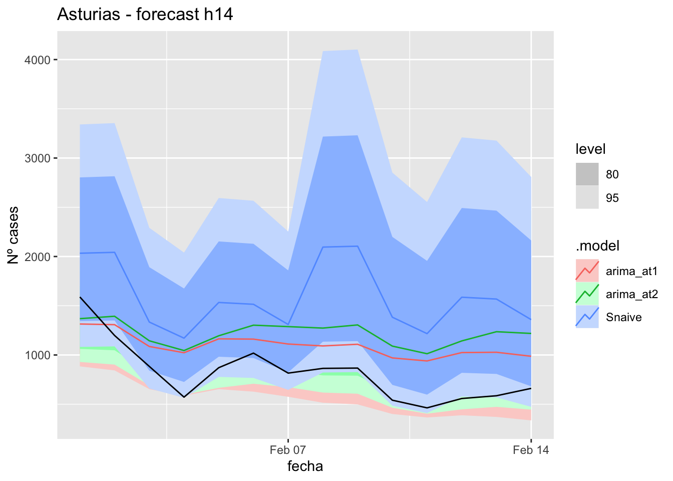
fc_h14 %>%
autoplot(
data_asturias %>%
filter(fecha <= as.Date("2022-01-31", format = "%Y-%m-%d")+days(14) &
fecha > as.Date("2022-01-01", format = "%Y-%m-%d"))
) +
labs(y = "Nº cases", title = "Asturias - forecast h14")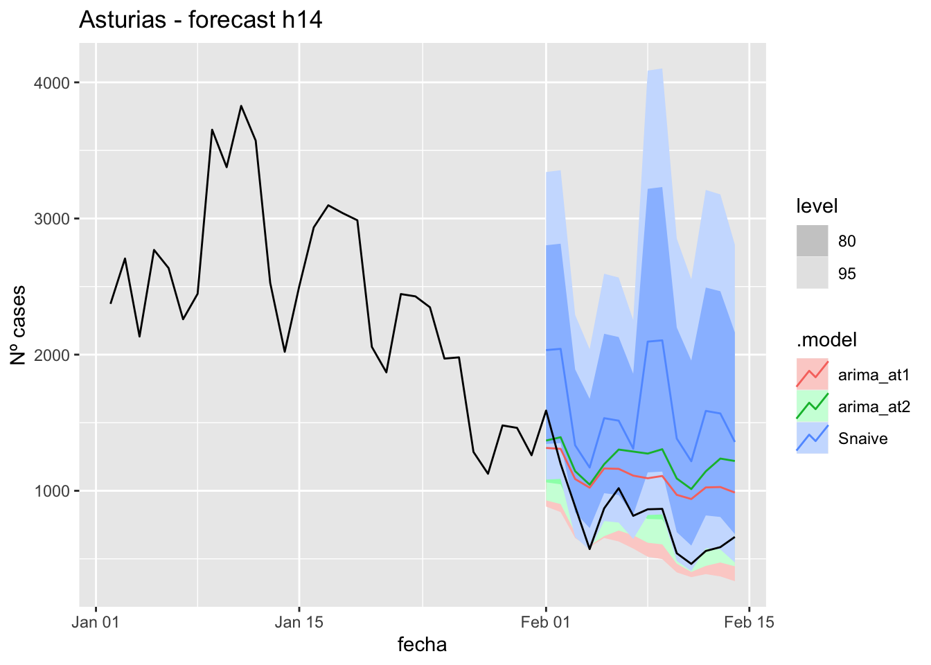
# Accuracy
fabletools::accuracy(fc_h14, data_asturias)# A tibble: 3 × 11
.model provincia .type ME RMSE MAE MPE MAPE MASE RMSSE ACF1
<chr> <chr> <chr> <dbl> <dbl> <dbl> <dbl> <dbl> <dbl> <dbl> <dbl>
1 arima_at1 Asturias Test -273. 334. 313. -44.4 46.9 3.23 1.52 0.375
2 arima_at2 Asturias Test -395. 449. 426. -61.1 63.1 4.40 2.04 0.443
3 Snaive Asturias Test -769. 812. 769. -107. 107. 7.94 3.69 0.29921 days
# Plots
fc_h21 %>%
autoplot(
data_asturias_test %>%
filter(fecha <= as.Date("2022-01-31", format = "%Y-%m-%d")+days(21))
) +
labs(y = "Nº cases", title = "Asturias - forecast h21")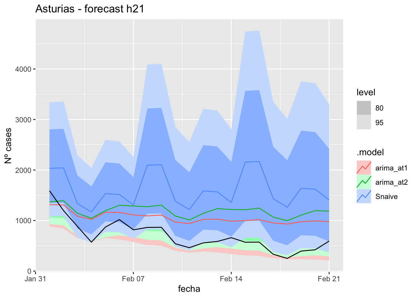
fc_h21 %>%
autoplot(
data_asturias %>%
filter(fecha <= as.Date("2022-01-31", format = "%Y-%m-%d")+days(21) &
fecha > as.Date("2022-01-01", format = "%Y-%m-%d"))
) +
labs(y = "Nº cases", title = "Asturias - forecast h21")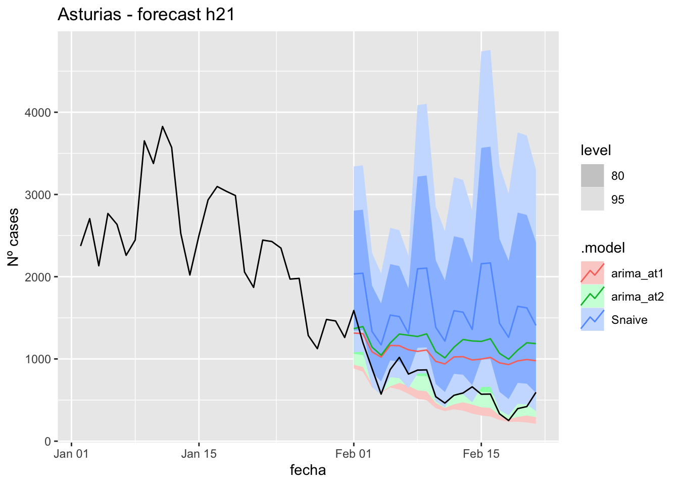
# Accuracy
fabletools::accuracy(fc_h21, data_asturias)# A tibble: 3 × 11
.model provincia .type ME RMSE MAE MPE MAPE MASE RMSSE ACF1
<chr> <chr> <chr> <dbl> <dbl> <dbl> <dbl> <dbl> <dbl> <dbl> <dbl>
1 arima_at1 Asturias Test -359. 414. 385. -75.2 76.8 3.98 1.88 0.534
2 arima_at2 Asturias Test -495. 545. 516. -98.4 99.8 5.34 2.48 0.595
3 Snaive Asturias Test -920. 980. 920. -168. 168. 9.50 4.46 0.43757 days
# Plots
fc_h57 %>%
autoplot(
data_asturias_test %>%
filter(fecha <= as.Date("2022-01-31", format = "%Y-%m-%d")+days(57))
) +
labs(y = "Nº cases", title = "Asturias - forecast h57")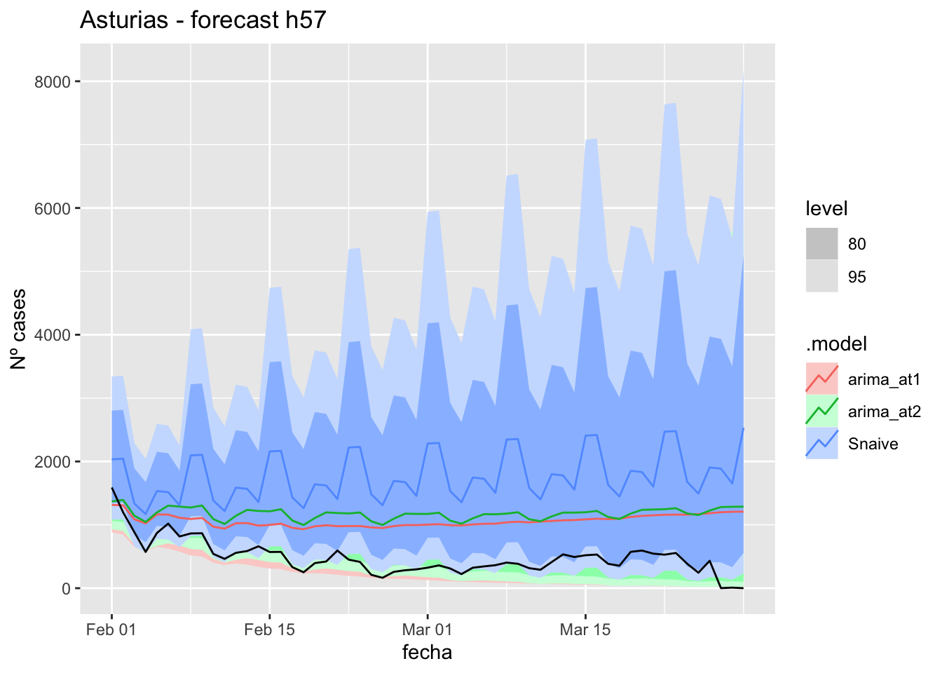
fc_h57 %>%
autoplot(
data_asturias %>%
filter(fecha <= as.Date("2022-01-31", format = "%Y-%m-%d")+days(57) &
fecha > as.Date("2022-01-01", format = "%Y-%m-%d"))
) +
labs(y = "Nº cases", title = "Asturias - forecast h57")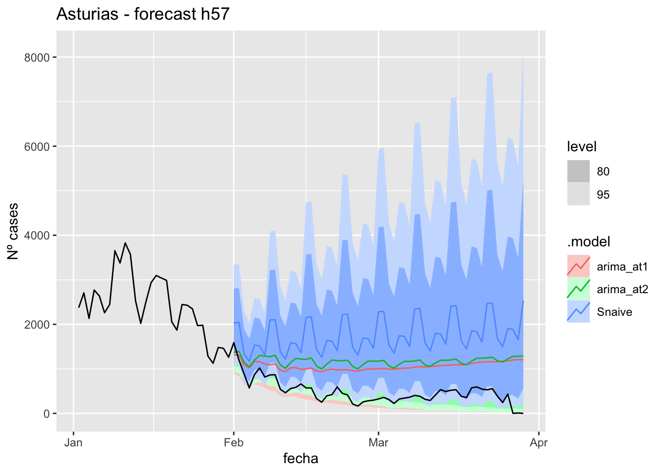
# Accuracy
fabletools::accuracy(fc_h57, data_asturias)# A tibble: 3 × 11
.model provincia .type ME RMSE MAE MPE MAPE MASE RMSSE ACF1
<chr> <chr> <chr> <dbl> <dbl> <dbl> <dbl> <dbl> <dbl> <dbl> <dbl>
1 arima_at1 Asturias Test -583. 634. 592. -Inf Inf 6.12 2.88 0.720
2 arima_at2 Asturias Test -694. 735. 702. -Inf Inf 7.25 3.34 0.712
3 Snaive Asturias Test -1282. 1359. 1282. -Inf Inf 13.3 6.18 0.471Barcelona
data_Barcelona <- covid_data %>%
filter(provincia == "Barcelona") %>%
filter(fecha > as.Date("2020-06-14", format = "%Y-%m-%d")) %>%
select(provincia, fecha, num_casos, tmed) %>%
drop_na() %>%
as_tsibble(key = provincia, index = fecha)
data_Barcelona# A tsibble: 653 x 4 [1D]
# Key: provincia [1]
provincia fecha num_casos tmed
<chr> <date> <dbl> <dbl>
1 Barcelona 2020-06-15 62 21.2
2 Barcelona 2020-06-16 66 20.8
3 Barcelona 2020-06-17 70 20.3
4 Barcelona 2020-06-18 68 18.8
5 Barcelona 2020-06-19 65 20.4
6 Barcelona 2020-06-20 53 21.8
7 Barcelona 2020-06-21 38 22.8
8 Barcelona 2020-06-22 69 23.8
9 Barcelona 2020-06-23 95 23.4
10 Barcelona 2020-06-24 44 23.6
# … with 643 more rowsdata_Barcelona_train <- data_Barcelona %>%
filter(fecha <= as.Date("2022-01-31", format = "%Y-%m-%d"))
summary(data_Barcelona_train$fecha) Min. 1st Qu. Median Mean 3rd Qu. Max.
"2020-06-15" "2020-11-10" "2021-04-08" "2021-04-08" "2021-09-04" "2022-01-31" data_Barcelona_test <- data_Barcelona %>%
filter(fecha > as.Date("2022-01-31", format = "%Y-%m-%d"))
summary(data_Barcelona_test$fecha) Min. 1st Qu. Median Mean 3rd Qu. Max.
"2022-02-01" "2022-02-15" "2022-03-01" "2022-03-01" "2022-03-15" "2022-03-29" # Lamba for num_casos
lambda_Barcelona_casos <- data_Barcelona %>%
features(num_casos, features = guerrero) %>%
pull(lambda_guerrero)
lambda_Barcelona_casos[1] 0.1434101# Lamba for average temp
lambda_Barcelona_tmed <- data_Barcelona %>%
features(tmed, features = guerrero) %>%
pull(lambda_guerrero)
lambda_Barcelona_tmed[1] 1.098957fit_model <- data_Barcelona_train %>%
model(
arima_at1 = ARIMA(box_cox(num_casos, lambda_Barcelona_casos) ~
box_cox(tmed, lambda_Barcelona_tmed)),
arima_at2 = ARIMA(box_cox(num_casos, lambda_Barcelona_casos) ~
box_cox(tmed, lambda_Barcelona_tmed),
stepwise = FALSE, approx = FALSE),
Snaive = SNAIVE(box_cox(num_casos, lambda_Barcelona_casos))
)
# Show and report model
fit_model# A mable: 1 x 4
# Key: provincia [1]
provincia arima_at1
<chr> <model>
1 Barcelona <LM w/ ARIMA(1,0,2)(0,1,1)[7] errors>
# … with 2 more variables: arima_at2 <model>, Snaive <model>glance(fit_model)# A tibble: 3 × 9
provincia .model sigma2 log_lik AIC AICc BIC ar_roots ma_roots
<chr> <chr> <dbl> <dbl> <dbl> <dbl> <dbl> <list> <list>
1 Barcelona arima_at1 0.342 -521. 1054. 1054. 1080. <cpl [1]> <cpl [9]>
2 Barcelona arima_at2 0.328 -510. 1035. 1035. 1070. <cpl [4]> <cpl [8]>
3 Barcelona Snaive 1.26 NA NA NA NA <NULL> <NULL> fit_model %>%
pivot_longer(-provincia,
names_to = ".model",
values_to = "orders") %>%
left_join(glance(fit_model), by = c("provincia", ".model")) %>%
arrange(AICc) %>%
select(.model:BIC)# A mable: 3 x 7
# Key: .model [3]
.model orders sigma2 log_lik AIC AICc BIC
<chr> <model> <dbl> <dbl> <dbl> <dbl> <dbl>
1 arima_… <LM w/ ARIMA(4,0,1)(0,1,1)[7] errors> 0.328 -510. 1035. 1035. 1070.
2 arima_… <LM w/ ARIMA(1,0,2)(0,1,1)[7] errors> 0.342 -521. 1054. 1054. 1080.
3 Snaive <SNAIVE> 1.26 NA NA NA NA # We use a Ljung-Box test >> large p-value, confirms residuals are similar / considered to white noise
fit_model %>%
select(Snaive) %>%
gg_tsresiduals()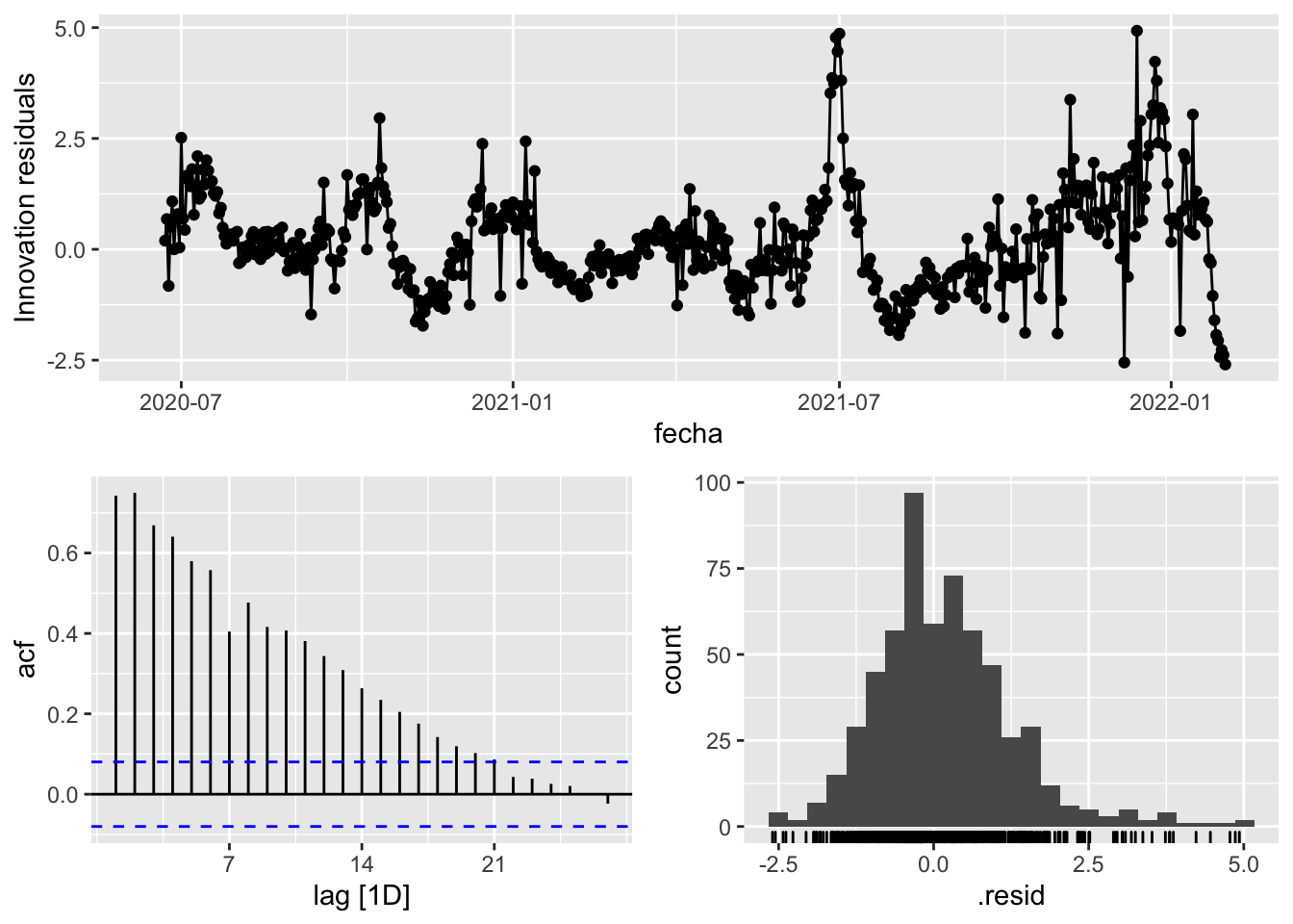
fit_model %>%
select(arima_at1) %>%
gg_tsresiduals()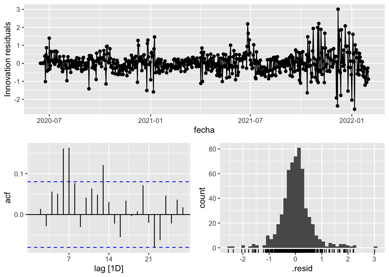
fit_model %>%
select(arima_at2) %>%
gg_tsresiduals()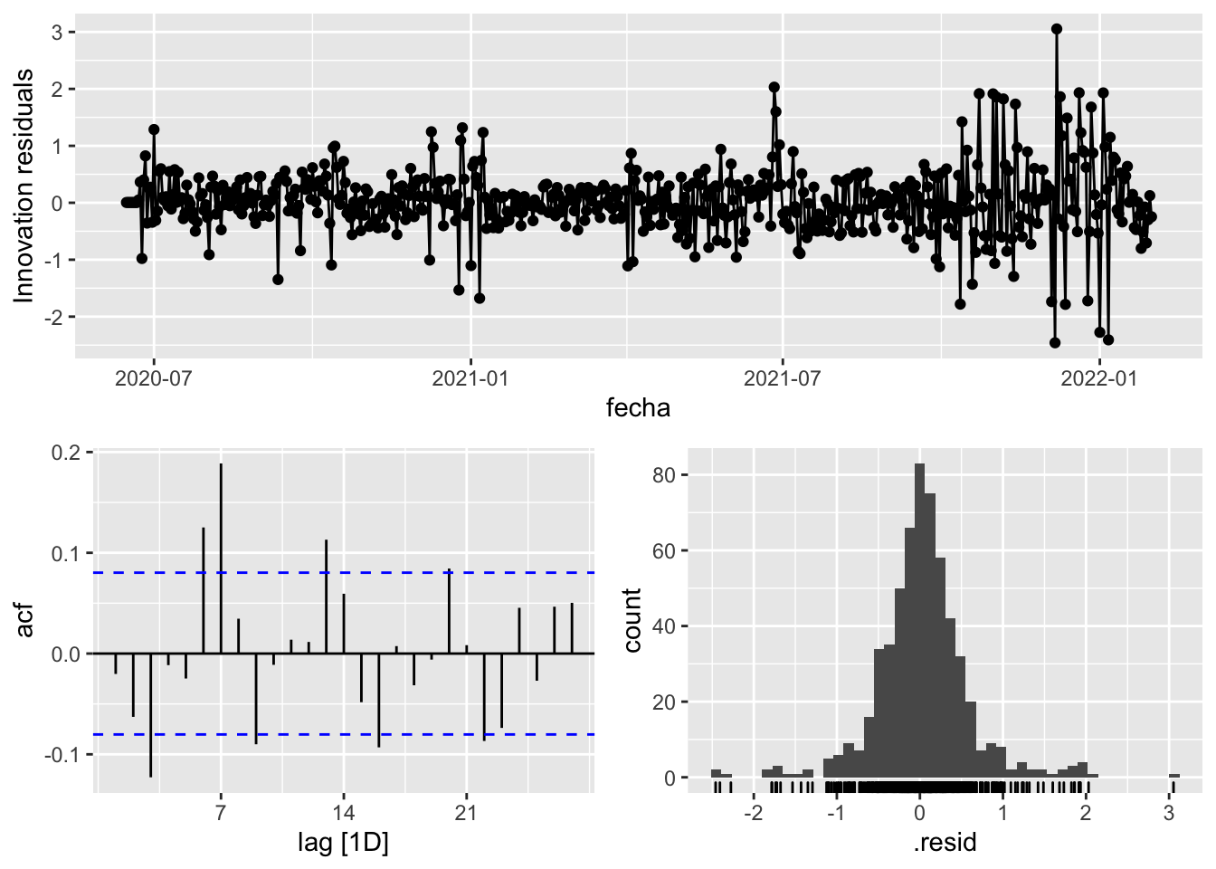
augment(fit_model) %>%
features(.innov, ljung_box, lag=7)# A tibble: 3 × 4
provincia .model lb_stat lb_pvalue
<chr> <chr> <dbl> <dbl>
1 Barcelona arima_at1 35.9 0.00000742
2 Barcelona arima_at2 43.1 0.000000313
3 Barcelona Snaive 1654. 0 augment(fit_model) %>%
features(.innov, ljung_box, lag=14)# A tibble: 3 × 4
provincia .model lb_stat lb_pvalue
<chr> <chr> <dbl> <dbl>
1 Barcelona arima_at1 54.6 0.00000102
2 Barcelona arima_at2 59.0 0.000000174
3 Barcelona Snaive 2253. 0 augment(fit_model) %>%
features(.innov, ljung_box, lag=21)# A tibble: 3 × 4
provincia .model lb_stat lb_pvalue
<chr> <chr> <dbl> <dbl>
1 Barcelona arima_at1 60.9 0.00000917
2 Barcelona arima_at2 70.9 0.000000253
3 Barcelona Snaive 2362. 0 augment(fit_model) %>%
features(.innov, ljung_box, lag=57)# A tibble: 3 × 4
provincia .model lb_stat lb_pvalue
<chr> <chr> <dbl> <dbl>
1 Barcelona arima_at1 164. 2.71e-12
2 Barcelona arima_at2 162. 4.88e-12
3 Barcelona Snaive 2651. 0 # To predict future values of infections, we need to pass the model future/prediction values of the complementary variables tmed and mobility
# We are going to select those from the test dataset
data_fc_h7 <- data_Barcelona_test %>%
select(-num_casos) %>%
slice(1:7)
data_fc_h14 <- data_Barcelona_test %>%
select(-num_casos) %>%
slice(1:14)
data_fc_h21 <- data_Barcelona_test %>%
select(-num_casos) %>%
slice(1:21)
data_fc_h57 <- data_Barcelona_test %>%
select(-num_casos) %>%
slice(1:57)# Significant spikes out of 30 is still consistent with white noise
# To be sure, use a Ljung-Box test, which has a large p-value, confirming that
# the residuals are similar to white noise.
# Note that the alternative models also passed this test.
#
# Forecast
fc_h7 <- fabletools::forecast(fit_model, new_data = data_fc_h7)
fc_h14 <- fabletools::forecast(fit_model, new_data = data_fc_h14)
fc_h21 <- fabletools::forecast(fit_model, new_data = data_fc_h21)
fc_h57 <- fabletools::forecast(fit_model, new_data = data_fc_h57)7 days
# Plots
fc_h7 %>%
autoplot(
data_Barcelona_test %>%
filter(fecha <= as.Date("2022-01-31", format = "%Y-%m-%d")+days(7))
) +
labs(y = "Nº cases", title = "Barcelona - forecast h7")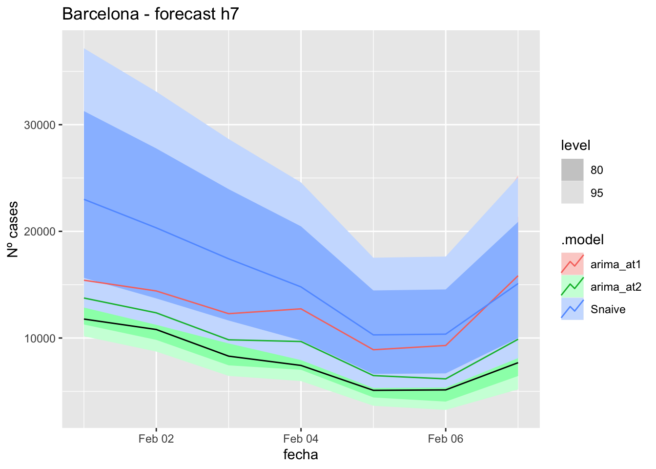
fc_h7 %>%
autoplot(
data_Barcelona %>%
filter(fecha <= as.Date("2022-01-31", format = "%Y-%m-%d")+days(7) &
fecha > as.Date("2022-01-01", format = "%Y-%m-%d"))
) +
labs(y = "Nº cases", title = "Barcelona - forecast h7")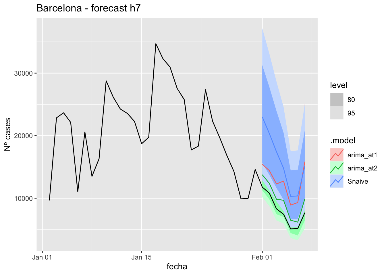
# Accuracy
fabletools::accuracy(fc_h7, data_Barcelona)# A tibble: 3 × 11
.model provincia .type ME RMSE MAE MPE MAPE MASE RMSSE ACF1
<chr> <chr> <chr> <dbl> <dbl> <dbl> <dbl> <dbl> <dbl> <dbl> <dbl>
1 arima_at1 Barcelona Test -4666. 4908. 4666. -63.7 63.7 5.86 2.51 -0.0314
2 arima_at2 Barcelona Test -1704. 1754. 1704. -22.3 22.3 2.14 0.896 -0.328
3 Snaive Barcelona Test -7870. 8139. 7870. -99.0 99.0 9.88 4.16 0.551 14 days
# Plots
fc_h14 %>%
autoplot(
data_Barcelona_test %>%
filter(fecha <= as.Date("2022-01-31", format = "%Y-%m-%d")+days(14))
) +
labs(y = "Nº cases", title = "Barcelona - forecast h14")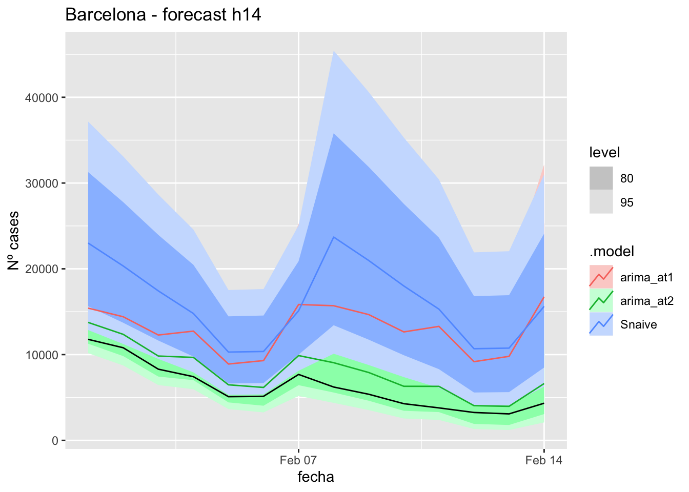
fc_h14 %>%
autoplot(
data_Barcelona %>%
filter(fecha <= as.Date("2022-01-31", format = "%Y-%m-%d")+days(14) &
fecha > as.Date("2022-01-01", format = "%Y-%m-%d"))
) +
labs(y = "Nº cases", title = "Barcelona - forecast h14")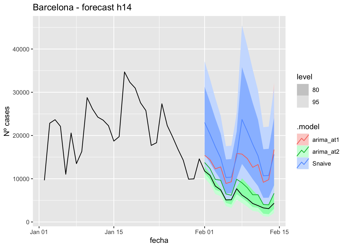
# Accuracy
fabletools::accuracy(fc_h14, data_Barcelona)# A tibble: 3 × 11
.model provincia .type ME RMSE MAE MPE MAPE MASE RMSSE ACF1
<chr> <chr> <chr> <dbl> <dbl> <dbl> <dbl> <dbl> <dbl> <dbl> <dbl>
1 arima_at1 Barcelona Test -6738. 7266. 6738. -136. 136. 8.46 3.71 0.459
2 arima_at2 Barcelona Test -1843. 1947. 1843. -33.4 33.4 2.31 0.994 0.180
3 Snaive Barcelona Test -9985. 10606. 9985. -188. 188. 12.5 5.42 0.54821 days
# Plots
fc_h21 %>%
autoplot(
data_Barcelona_test %>%
filter(fecha <= as.Date("2022-01-31", format = "%Y-%m-%d")+days(21))
) +
labs(y = "Nº cases", title = "Barcelona - forecast h21")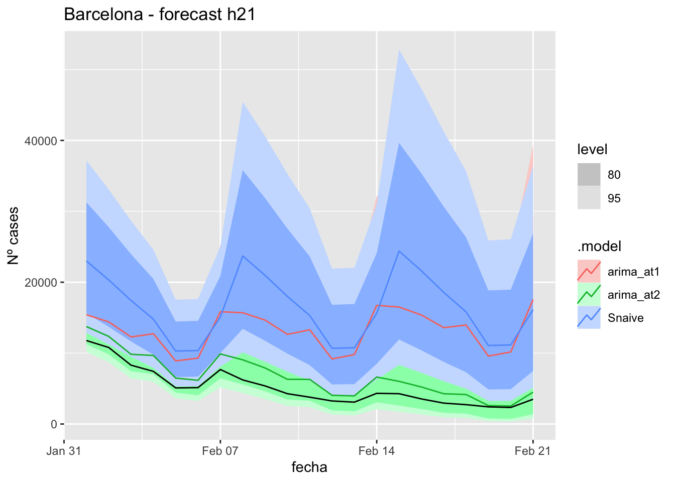
fc_h21 %>%
autoplot(
data_Barcelona %>%
filter(fecha <= as.Date("2022-01-31", format = "%Y-%m-%d")+days(21) &
fecha > as.Date("2022-01-01", format = "%Y-%m-%d"))
) +
labs(y = "Nº cases", title = "Barcelona - forecast h21")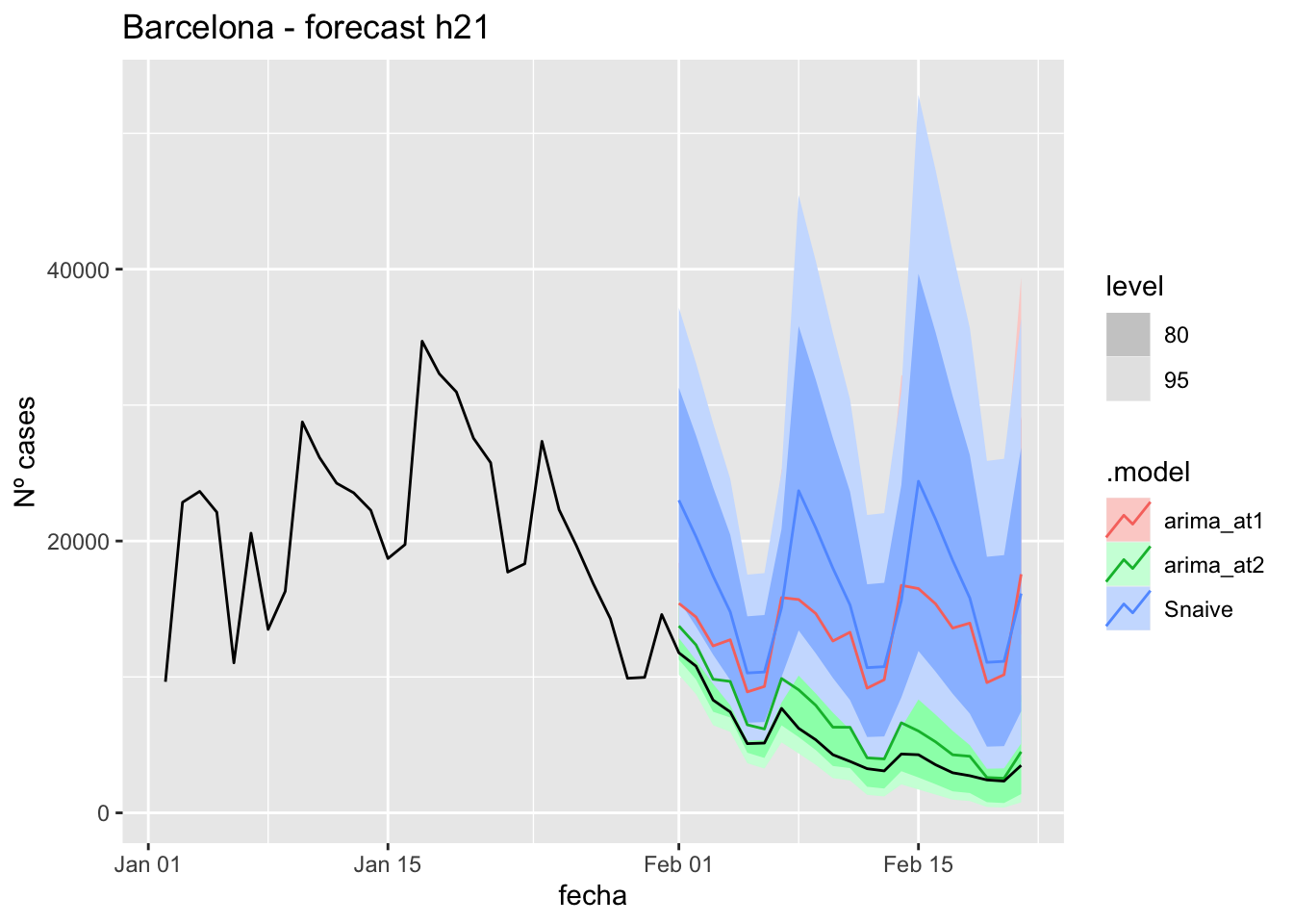
# Accuracy
fabletools::accuracy(fc_h21, data_Barcelona)# A tibble: 3 × 11
.model provincia .type ME RMSE MAE MPE MAPE MASE RMSSE ACF1
<chr> <chr> <chr> <dbl> <dbl> <dbl> <dbl> <dbl> <dbl> <dbl> <dbl>
1 arima_at1 Barcelona Test -8063. 8669. 8063. -206. 206. 10.1 4.43 0.569
2 arima_at2 Barcelona Test -1589. 1743. 1589. -33.3 33.3 2.00 0.890 0.446
3 Snaive Barcelona Test -11275. 12018. 11275. -272. 272. 14.2 6.14 0.60257 days
# Plots
fc_h57 %>%
autoplot(
data_Barcelona_test %>%
filter(fecha <= as.Date("2022-01-31", format = "%Y-%m-%d")+days(57))
) +
labs(y = "Nº cases", title = "Barcelona - forecast h57")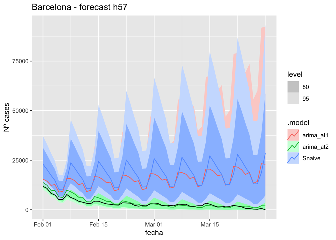
fc_h57 %>%
autoplot(
data_Barcelona %>%
filter(fecha <= as.Date("2022-01-31", format = "%Y-%m-%d")+days(57) &
fecha > as.Date("2022-01-01", format = "%Y-%m-%d"))
) +
labs(y = "Nº cases", title = "Barcelona - forecast h57")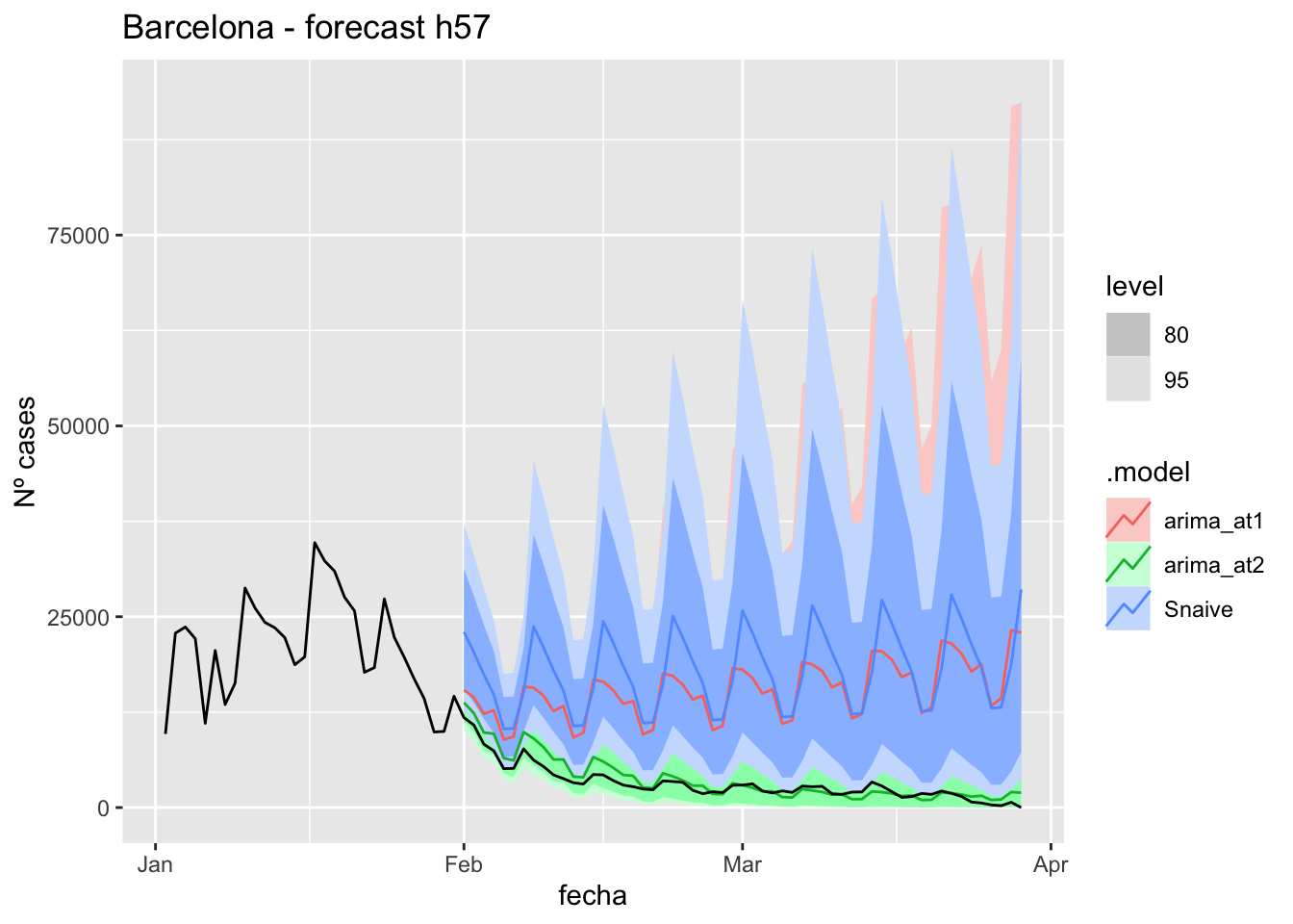
# Accuracy
fabletools::accuracy(fc_h57, data_Barcelona)# A tibble: 3 × 11
.model provincia .type ME RMSE MAE MPE MAPE MASE RMSSE ACF1
<chr> <chr> <chr> <dbl> <dbl> <dbl> <dbl> <dbl> <dbl> <dbl> <dbl>
1 arima_at1 Barcelona Test -12180. 13056. 12180. -Inf Inf 15.3 6.67 0.704
2 arima_at2 Barcelona Test -582. 1198. 942. -Inf Inf 1.18 0.612 0.806
3 Snaive Barcelona Test -14809. 15796. 14809. -Inf Inf 18.6 8.06 0.592Madrid
data_Madrid <- covid_data %>%
filter(provincia == "Madrid") %>%
filter(fecha > as.Date("2020-06-14", format = "%Y-%m-%d")) %>%
select(provincia, fecha, num_casos, tmed) %>%
drop_na() %>%
as_tsibble(key = provincia, index = fecha)
data_Madrid# A tsibble: 653 x 4 [1D]
# Key: provincia [1]
provincia fecha num_casos tmed
<chr> <date> <dbl> <dbl>
1 Madrid 2020-06-15 153 20.7
2 Madrid 2020-06-16 91 21
3 Madrid 2020-06-17 93 20.2
4 Madrid 2020-06-18 85 21.9
5 Madrid 2020-06-19 78 22.6
6 Madrid 2020-06-20 67 23.4
7 Madrid 2020-06-21 42 25
8 Madrid 2020-06-22 60 27.3
9 Madrid 2020-06-23 68 28.4
10 Madrid 2020-06-24 49 28
# … with 643 more rowsdata_Madrid_train <- data_Madrid %>%
filter(fecha <= as.Date("2022-01-31", format = "%Y-%m-%d"))
summary(data_Madrid_train$fecha) Min. 1st Qu. Median Mean 3rd Qu. Max.
"2020-06-15" "2020-11-10" "2021-04-08" "2021-04-08" "2021-09-04" "2022-01-31" data_Madrid_test <- data_Madrid %>%
filter(fecha > as.Date("2022-01-31", format = "%Y-%m-%d"))
summary(data_Madrid_test$fecha) Min. 1st Qu. Median Mean 3rd Qu. Max.
"2022-02-01" "2022-02-15" "2022-03-01" "2022-03-01" "2022-03-15" "2022-03-29" # Lamba for num_casos
lambda_Madrid_casos <- data_Madrid %>%
features(num_casos, features = guerrero) %>%
pull(lambda_guerrero)
lambda_Madrid_casos[1] 0.06260614# Lamba for average temp
lambda_Madrid_tmed <- data_Madrid %>%
features(tmed, features = guerrero) %>%
pull(lambda_guerrero)
lambda_Madrid_tmed[1] 0.936519fit_model <- data_Madrid_train %>%
model(
arima_at1 = ARIMA(box_cox(num_casos, lambda_Madrid_casos) ~
box_cox(tmed, lambda_Madrid_tmed)),
arima_at2 = ARIMA(box_cox(num_casos, lambda_Madrid_casos) ~
box_cox(tmed, lambda_Madrid_tmed),
stepwise = FALSE, approx = FALSE),
Snaive = SNAIVE(box_cox(num_casos, lambda_Madrid_casos))
)
# Show and report model
fit_model# A mable: 1 x 4
# Key: provincia [1]
provincia arima_at1
<chr> <model>
1 Madrid <LM w/ ARIMA(2,0,2)(0,1,2)[7] errors>
# … with 2 more variables: arima_at2 <model>, Snaive <model>glance(fit_model)# A tibble: 3 × 9
provincia .model sigma2 log_lik AIC AICc BIC ar_roots ma_roots
<chr> <chr> <dbl> <dbl> <dbl> <dbl> <dbl> <list> <list>
1 Madrid arima_at1 0.133 -240. 496. 496. 531. <cpl [2]> <cpl [16]>
2 Madrid arima_at2 0.133 -240. 496. 496. 531. <cpl [2]> <cpl [16]>
3 Madrid Snaive 0.412 NA NA NA NA <NULL> <NULL> fit_model %>%
pivot_longer(-provincia,
names_to = ".model",
values_to = "orders") %>%
left_join(glance(fit_model), by = c("provincia", ".model")) %>%
arrange(AICc) %>%
select(.model:BIC)# A mable: 3 x 7
# Key: .model [3]
.model orders sigma2 log_lik AIC AICc BIC
<chr> <model> <dbl> <dbl> <dbl> <dbl> <dbl>
1 arima_… <LM w/ ARIMA(2,0,2)(0,1,2)[7] errors> 0.133 -240. 496. 496. 531.
2 arima_… <LM w/ ARIMA(2,0,2)(0,1,2)[7] errors> 0.133 -240. 496. 496. 531.
3 Snaive <SNAIVE> 0.412 NA NA NA NA # We use a Ljung-Box test >> large p-value, confirms residuals are similar / considered to white noise
fit_model %>%
select(Snaive) %>%
gg_tsresiduals()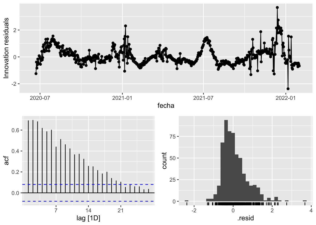
fit_model %>%
select(arima_at1) %>%
gg_tsresiduals()
fit_model %>%
select(arima_at2) %>%
gg_tsresiduals()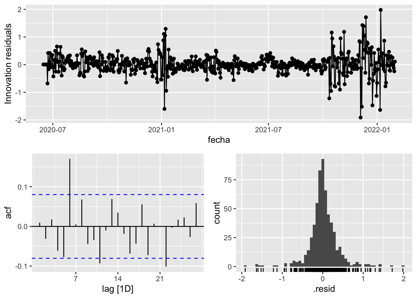
augment(fit_model) %>%
features(.innov, ljung_box, lag=7)# A tibble: 3 × 4
provincia .model lb_stat lb_pvalue
<chr> <chr> <dbl> <dbl>
1 Madrid arima_at1 24.2 0.00104
2 Madrid arima_at2 24.2 0.00104
3 Madrid Snaive 1617. 0 augment(fit_model) %>%
features(.innov, ljung_box, lag=14)# A tibble: 3 × 4
provincia .model lb_stat lb_pvalue
<chr> <chr> <dbl> <dbl>
1 Madrid arima_at1 37.9 0.000530
2 Madrid arima_at2 37.9 0.000530
3 Madrid Snaive 2282. 0 augment(fit_model) %>%
features(.innov, ljung_box, lag=21)# A tibble: 3 × 4
provincia .model lb_stat lb_pvalue
<chr> <chr> <dbl> <dbl>
1 Madrid arima_at1 47.4 0.000825
2 Madrid arima_at2 47.4 0.000825
3 Madrid Snaive 2422. 0 augment(fit_model) %>%
features(.innov, ljung_box, lag=57)# A tibble: 3 × 4
provincia .model lb_stat lb_pvalue
<chr> <chr> <dbl> <dbl>
1 Madrid arima_at1 122. 0.00000139
2 Madrid arima_at2 122. 0.00000139
3 Madrid Snaive 2762. 0 # To predict future values of infections, we need to pass the model future/prediction values of the complementary variables tmed and mobility
# We are going to select those from the test dataset
data_fc_h7 <- data_Madrid_test %>%
select(-num_casos) %>%
slice(1:7)
data_fc_h14 <- data_Madrid_test %>%
select(-num_casos) %>%
slice(1:14)
data_fc_h21 <- data_Madrid_test %>%
select(-num_casos) %>%
slice(1:21)
data_fc_h57 <- data_Madrid_test %>%
select(-num_casos) %>%
slice(1:57)# Significant spikes out of 30 is still consistent with white noise
# To be sure, use a Ljung-Box test, which has a large p-value, confirming that
# the residuals are similar to white noise.
# Note that the alternative models also passed this test.
#
# Forecast
fc_h7 <- fabletools::forecast(fit_model, new_data = data_fc_h7)
fc_h14 <- fabletools::forecast(fit_model, new_data = data_fc_h14)
fc_h21 <- fabletools::forecast(fit_model, new_data = data_fc_h21)
fc_h57 <- fabletools::forecast(fit_model, new_data = data_fc_h57)7 days
# Plots
fc_h7 %>%
autoplot(
data_Madrid_test %>%
filter(fecha <= as.Date("2022-01-31", format = "%Y-%m-%d")+days(7))
) +
labs(y = "Nº cases", title = "Madrid - forecast h7")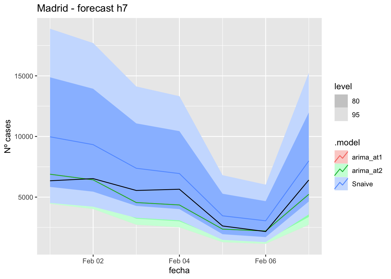
fc_h7 %>%
autoplot(
data_Madrid %>%
filter(fecha <= as.Date("2022-01-31", format = "%Y-%m-%d")+days(7) &
fecha > as.Date("2022-01-01", format = "%Y-%m-%d"))
) +
labs(y = "Nº cases", title = "Madrid - forecast h7")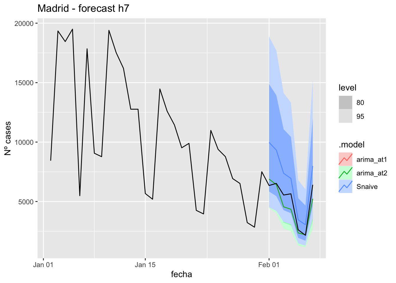
# Accuracy
fabletools::accuracy(fc_h7, data_Madrid)# A tibble: 3 × 11
.model provincia .type ME RMSE MAE MPE MAPE MASE RMSSE ACF1
<chr> <chr> <chr> <dbl> <dbl> <dbl> <dbl> <dbl> <dbl> <dbl> <dbl>
1 arima_at1 Madrid Test 464. 796. 632. 8.60 11.7 0.846 0.446 0.0623
2 arima_at2 Madrid Test 464. 796. 632. 8.60 11.7 0.846 0.446 0.0623
3 Snaive Madrid Test -1836. 2070. 1836. -36.2 36.2 2.46 1.16 0.541 14 days
# Plots
fc_h14 %>%
autoplot(
data_Madrid_test %>%
filter(fecha <= as.Date("2022-01-31", format = "%Y-%m-%d")+days(14))
) +
labs(y = "Nº cases", title = "Madrid - forecast h14")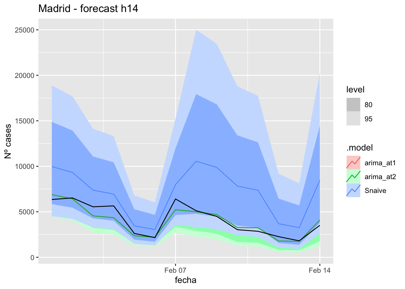
fc_h14 %>%
autoplot(
data_Madrid %>%
filter(fecha <= as.Date("2022-01-31", format = "%Y-%m-%d")+days(14) &
fecha > as.Date("2022-01-01", format = "%Y-%m-%d"))
) +
labs(y = "Nº cases", title = "Madrid - forecast h14")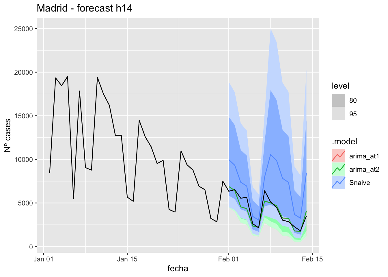
# Accuracy
fabletools::accuracy(fc_h14, data_Madrid)# A tibble: 3 × 11
.model provincia .type ME RMSE MAE MPE MAPE MASE RMSSE ACF1
<chr> <chr> <chr> <dbl> <dbl> <dbl> <dbl> <dbl> <dbl> <dbl> <dbl>
1 arima_at1 Madrid Test 179. 613. 463. 3.20 10.8 0.620 0.343 0.206
2 arima_at2 Madrid Test 179. 613. 463. 3.20 10.8 0.620 0.343 0.206
3 Snaive Madrid Test -2914. 3386. 2914. -77.1 77.1 3.90 1.90 0.46621 days
# Plots
fc_h21 %>%
autoplot(
data_Madrid_test %>%
filter(fecha <= as.Date("2022-01-31", format = "%Y-%m-%d")+days(21))
) +
labs(y = "Nº cases", title = "Madrid - forecast h21")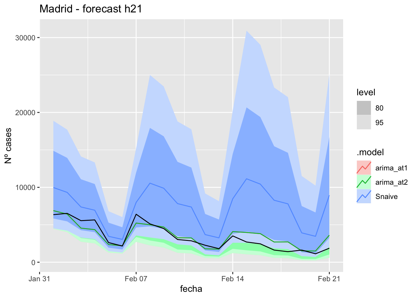
fc_h21 %>%
autoplot(
data_Madrid %>%
filter(fecha <= as.Date("2022-01-31", format = "%Y-%m-%d")+days(21) &
fecha > as.Date("2022-01-01", format = "%Y-%m-%d"))
) +
labs(y = "Nº cases", title = "Madrid - forecast h21")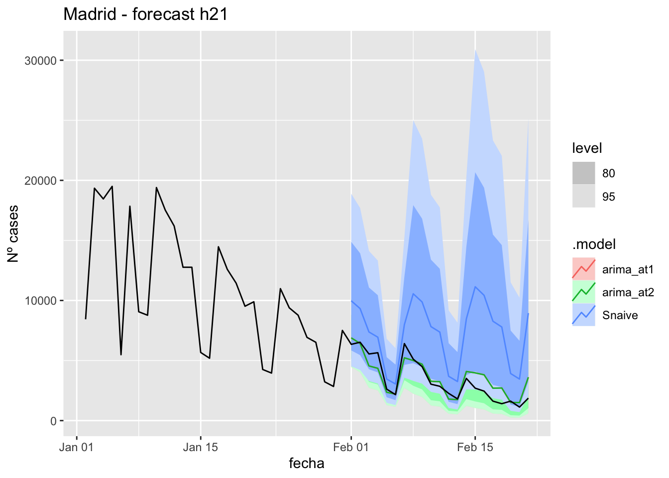
# Accuracy
fabletools::accuracy(fc_h21, data_Madrid)# A tibble: 3 × 11
.model provincia .type ME RMSE MAE MPE MAPE MASE RMSSE ACF1
<chr> <chr> <chr> <dbl> <dbl> <dbl> <dbl> <dbl> <dbl> <dbl> <dbl>
1 arima_at1 Madrid Test -216. 839. 654. -16.1 26.0 0.875 0.470 0.503
2 arima_at2 Madrid Test -216. 839. 654. -16.1 26.0 0.875 0.470 0.503
3 Snaive Madrid Test -3903. 4584. 3903. -158. 158. 5.23 2.57 0.57457 days
# Plots
fc_h57 %>%
autoplot(
data_Madrid_test %>%
filter(fecha <= as.Date("2022-01-31", format = "%Y-%m-%d")+days(57))
) +
labs(y = "Nº cases", title = "Madrid - forecast h57")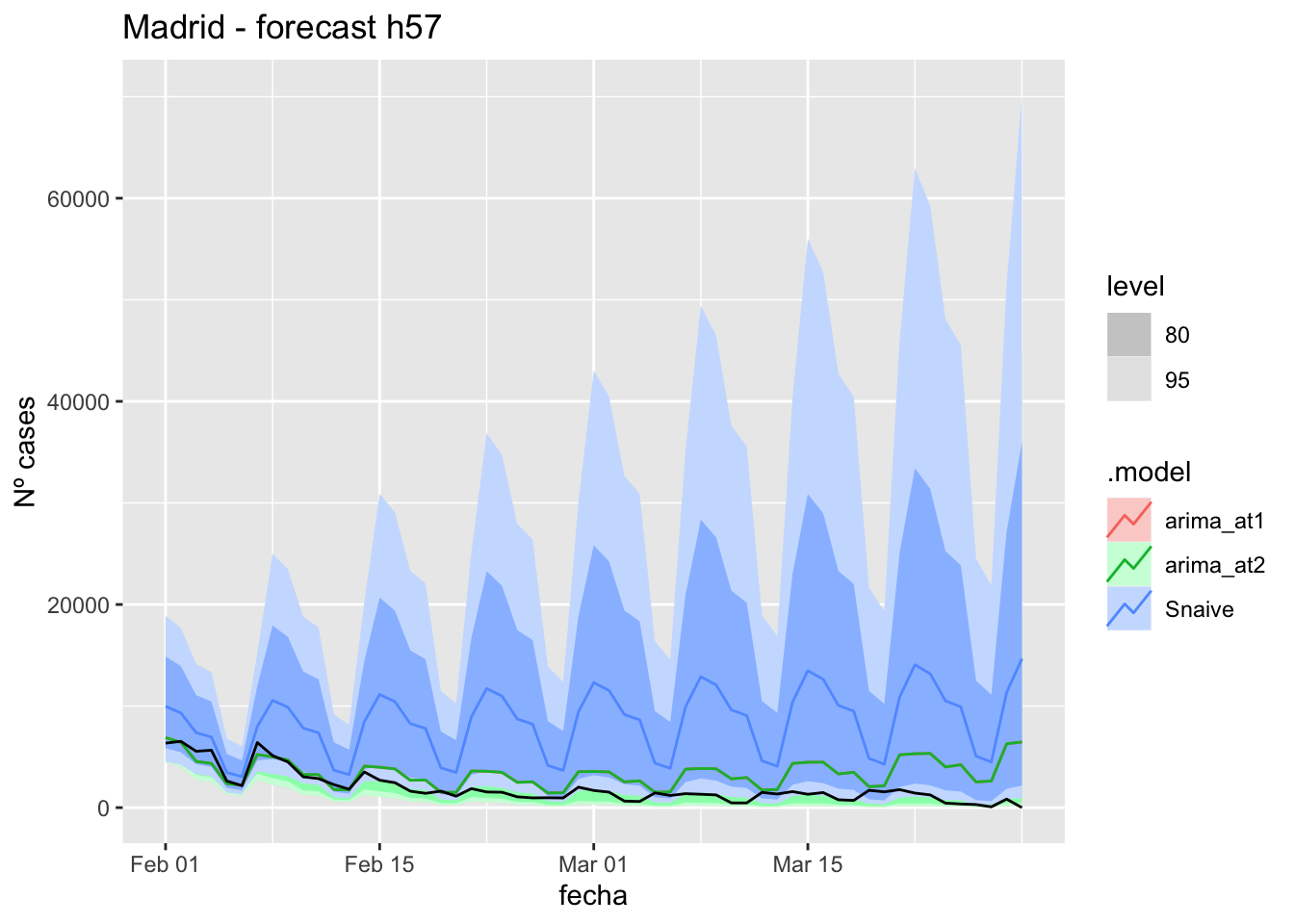
fc_h57 %>%
autoplot(
data_Madrid %>%
filter(fecha <= as.Date("2022-01-31", format = "%Y-%m-%d")+days(57) &
fecha > as.Date("2022-01-01", format = "%Y-%m-%d"))
) +
labs(y = "Nº cases", title = "Madrid - forecast h57")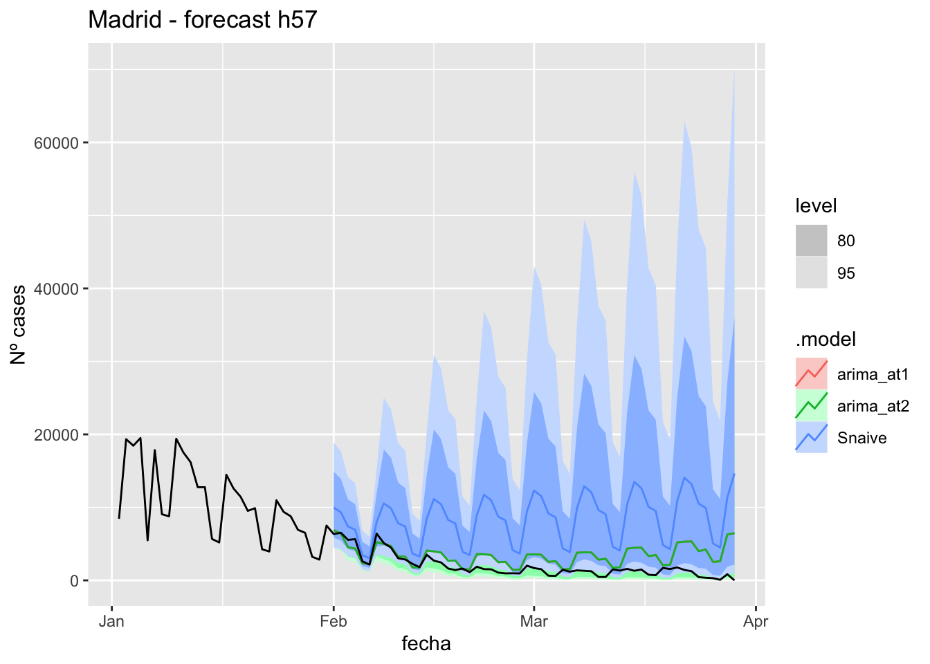
# Accuracy
fabletools::accuracy(fc_h57, data_Madrid)# A tibble: 3 × 11
.model provincia .type ME RMSE MAE MPE MAPE MASE RMSSE ACF1
<chr> <chr> <chr> <dbl> <dbl> <dbl> <dbl> <dbl> <dbl> <dbl> <dbl>
1 arima_at1 Madrid Test -1509. 2183. 1670. -2106. 2110. 2.24 1.22 0.698
2 arima_at2 Madrid Test -1509. 2183. 1670. -2106. 2110. 2.24 1.22 0.698
3 Snaive Madrid Test -6507. 7446. 6507. -4965. 4965. 8.71 4.17 0.627Malaga
data_Malaga <- covid_data %>%
filter(provincia == "Málaga") %>%
filter(fecha > as.Date("2020-06-14", format = "%Y-%m-%d")) %>%
select(provincia, fecha, num_casos, tmed) %>%
drop_na() %>%
as_tsibble(key = provincia, index = fecha)
data_Malaga# A tsibble: 653 x 4 [1D]
# Key: provincia [1]
provincia fecha num_casos tmed
<chr> <date> <dbl> <dbl>
1 Málaga 2020-06-15 1 27.2
2 Málaga 2020-06-16 1 27.8
3 Málaga 2020-06-17 2 26.9
4 Málaga 2020-06-18 2 21.6
5 Málaga 2020-06-19 1 24.7
6 Málaga 2020-06-20 4 22.6
7 Málaga 2020-06-21 4 22.7
8 Málaga 2020-06-22 6 25
9 Málaga 2020-06-23 8 25.6
10 Málaga 2020-06-24 65 24.5
# … with 643 more rowsdata_Malaga_train <- data_Malaga %>%
filter(fecha <= as.Date("2022-01-31", format = "%Y-%m-%d"))
summary(data_Malaga_train$fecha) Min. 1st Qu. Median Mean 3rd Qu. Max.
"2020-06-15" "2020-11-10" "2021-04-08" "2021-04-08" "2021-09-04" "2022-01-31" data_Malaga_test <- data_Malaga %>%
filter(fecha > as.Date("2022-01-31", format = "%Y-%m-%d"))
summary(data_Malaga_test$fecha) Min. 1st Qu. Median Mean 3rd Qu. Max.
"2022-02-01" "2022-02-15" "2022-03-01" "2022-03-01" "2022-03-15" "2022-03-29" # Lamba for num_casos
lambda_Malaga_casos <- data_Malaga %>%
features(num_casos, features = guerrero) %>%
pull(lambda_guerrero)
lambda_Malaga_casos[1] 0.2312255# Lamba for average temp
lambda_Malaga_tmed <- data_Malaga %>%
features(tmed, features = guerrero) %>%
pull(lambda_guerrero)
lambda_Malaga_tmed[1] 0.6288527fit_model <- data_Malaga_train %>%
model(
arima_at1 = ARIMA(box_cox(num_casos, lambda_Malaga_casos) ~
box_cox(tmed, lambda_Malaga_tmed)),
arima_at2 = ARIMA(box_cox(num_casos, lambda_Malaga_casos) ~
box_cox(tmed, lambda_Malaga_tmed),
stepwise = FALSE, approx = FALSE),
Snaive = SNAIVE(box_cox(num_casos, lambda_Malaga_casos))
)
# Show and report model
fit_model# A mable: 1 x 4
# Key: provincia [1]
provincia arima_at1
<chr> <model>
1 Málaga <LM w/ ARIMA(4,1,0)(2,0,0)[7] errors>
# … with 2 more variables: arima_at2 <model>, Snaive <model>glance(fit_model)# A tibble: 3 × 9
provincia .model sigma2 log_lik AIC AICc BIC ar_roots ma_roots
<chr> <chr> <dbl> <dbl> <dbl> <dbl> <dbl> <list> <list>
1 Málaga arima_at1 0.650 -715. 1446. 1446. 1481. <cpl [18]> <cpl [0]>
2 Málaga arima_at2 0.628 -706. 1425. 1425. 1456. <cpl [10]> <cpl [7]>
3 Málaga Snaive 2.41 NA NA NA NA <NULL> <NULL> fit_model %>%
pivot_longer(-provincia,
names_to = ".model",
values_to = "orders") %>%
left_join(glance(fit_model), by = c("provincia", ".model")) %>%
arrange(AICc) %>%
select(.model:BIC)# A mable: 3 x 7
# Key: .model [3]
.model orders sigma2 log_lik AIC AICc BIC
<chr> <model> <dbl> <dbl> <dbl> <dbl> <dbl>
1 arima_… <LM w/ ARIMA(3,1,0)(1,0,1)[7] errors> 0.628 -706. 1425. 1425. 1456.
2 arima_… <LM w/ ARIMA(4,1,0)(2,0,0)[7] errors> 0.650 -715. 1446. 1446. 1481.
3 Snaive <SNAIVE> 2.41 NA NA NA NA # We use a Ljung-Box test >> large p-value, confirms residuals are similar / considered to white noise
fit_model %>%
select(Snaive) %>%
gg_tsresiduals()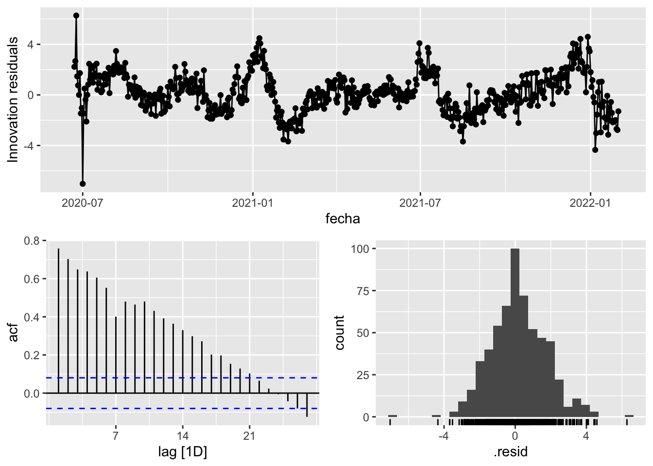
fit_model %>%
select(arima_at1) %>%
gg_tsresiduals()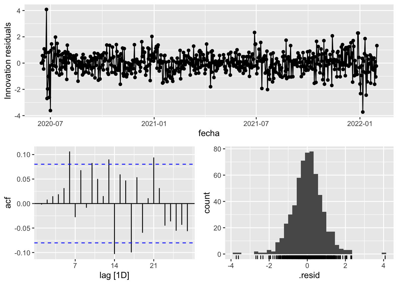
fit_model %>%
select(arima_at2) %>%
gg_tsresiduals()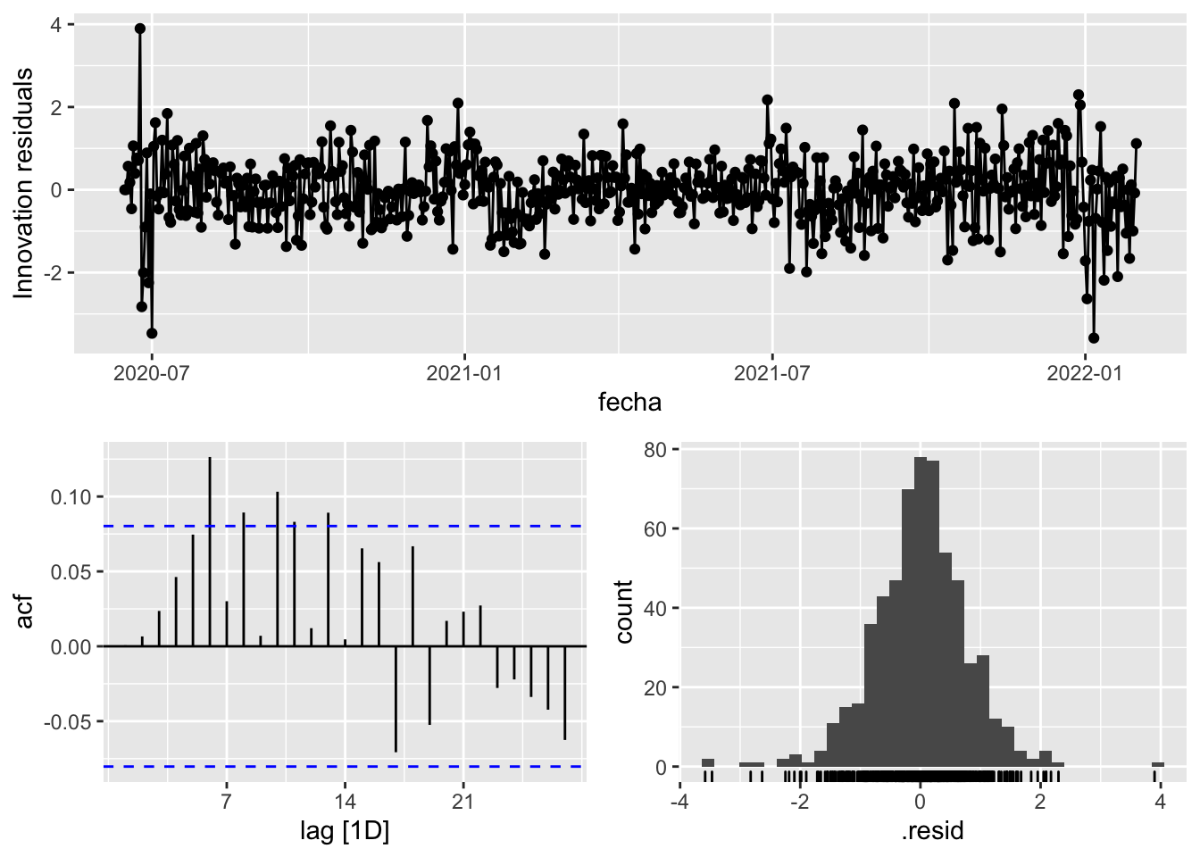
augment(fit_model) %>%
features(.innov, ljung_box, lag=7)# A tibble: 3 × 4
provincia .model lb_stat lb_pvalue
<chr> <chr> <dbl> <dbl>
1 Málaga arima_at1 8.29 0.308
2 Málaga arima_at2 15.2 0.0335
3 Málaga Snaive 1621. 0 augment(fit_model) %>%
features(.innov, ljung_box, lag=14)# A tibble: 3 × 4
provincia .model lb_stat lb_pvalue
<chr> <chr> <dbl> <dbl>
1 Málaga arima_at1 28.4 0.0124
2 Málaga arima_at2 35.7 0.00115
3 Málaga Snaive 2376. 0 augment(fit_model) %>%
features(.innov, ljung_box, lag=21)# A tibble: 3 × 4
provincia .model lb_stat lb_pvalue
<chr> <chr> <dbl> <dbl>
1 Málaga arima_at1 47.6 0.000771
2 Málaga arima_at2 48.3 0.000621
3 Málaga Snaive 2555. 0 augment(fit_model) %>%
features(.innov, ljung_box, lag=57)# A tibble: 3 × 4
provincia .model lb_stat lb_pvalue
<chr> <chr> <dbl> <dbl>
1 Málaga arima_at1 100. 0.000338
2 Málaga arima_at2 112. 0.0000197
3 Málaga Snaive 3422. 0 # To predict future values of infections, we need to pass the model future/prediction values of the complementary variables tmed and mobility
# We are going to select those from the test dataset
data_fc_h7 <- data_Malaga_test %>%
select(-num_casos) %>%
slice(1:7)
data_fc_h14 <- data_Malaga_test %>%
select(-num_casos) %>%
slice(1:14)
data_fc_h21 <- data_Malaga_test %>%
select(-num_casos) %>%
slice(1:21)
data_fc_h57 <- data_Malaga_test %>%
select(-num_casos) %>%
slice(1:57)# Significant spikes out of 30 is still consistent with white noise
# To be sure, use a Ljung-Box test, which has a large p-value, confirming that
# the residuals are similar to white noise.
# Note that the alternative models also passed this test.
#
# Forecast
fc_h7 <- fabletools::forecast(fit_model, new_data = data_fc_h7)
fc_h14 <- fabletools::forecast(fit_model, new_data = data_fc_h14)
fc_h21 <- fabletools::forecast(fit_model, new_data = data_fc_h21)
fc_h57 <- fabletools::forecast(fit_model, new_data = data_fc_h57)7 days
# Plots
fc_h7 %>%
autoplot(
data_Malaga_test %>%
filter(fecha <= as.Date("2022-01-31", format = "%Y-%m-%d")+days(7))
) +
labs(y = "Nº cases", title = "Malaga - forecast h7")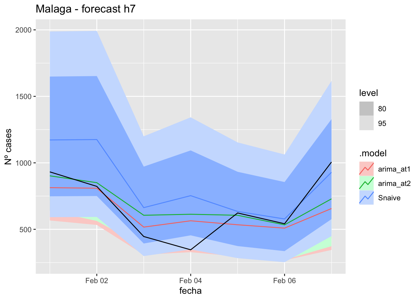
fc_h7 %>%
autoplot(
data_Malaga %>%
filter(fecha <= as.Date("2022-01-31", format = "%Y-%m-%d")+days(7) &
fecha > as.Date("2022-01-01", format = "%Y-%m-%d"))
) +
labs(y = "Nº cases", title = "Malaga - forecast h7")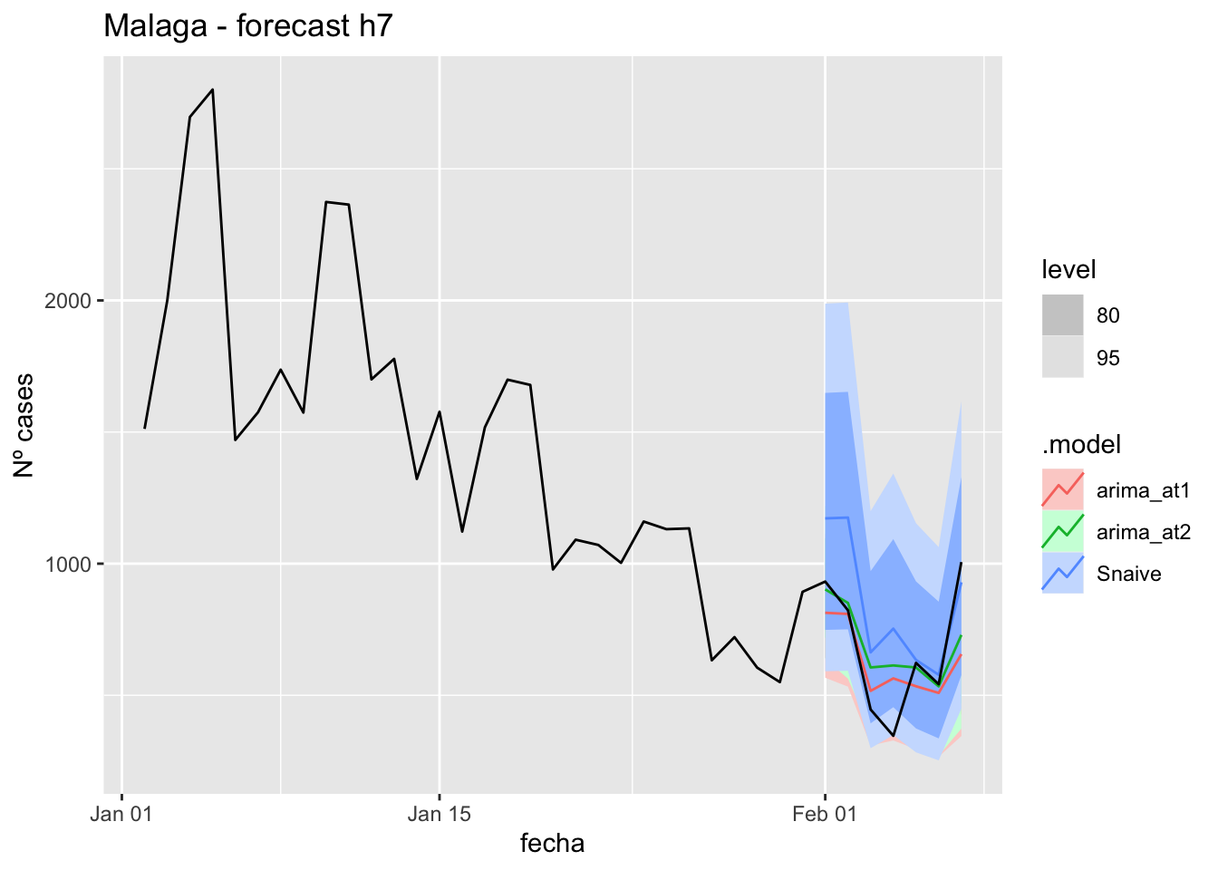
# Accuracy
fabletools::accuracy(fc_h7, data_Malaga)# A tibble: 3 × 11
.model provincia .type ME RMSE MAE MPE MAPE MASE RMSSE ACF1
<chr> <chr> <chr> <dbl> <dbl> <dbl> <dbl> <dbl> <dbl> <dbl> <dbl>
1 arima_at1 Málaga Test 45.0 168. 128. -1.35 21.2 0.965 0.680 0.0875
2 arima_at2 Málaga Test -17.6 158. 112. -11.6 21.6 0.851 0.640 0.209
3 Snaive Málaga Test -170. 240. 191. -33.7 35.9 1.45 0.968 0.246 14 days
# Plots
fc_h14 %>%
autoplot(
data_Malaga_test %>%
filter(fecha <= as.Date("2022-01-31", format = "%Y-%m-%d")+days(14))
) +
labs(y = "Nº cases", title = "Malaga - forecast h14")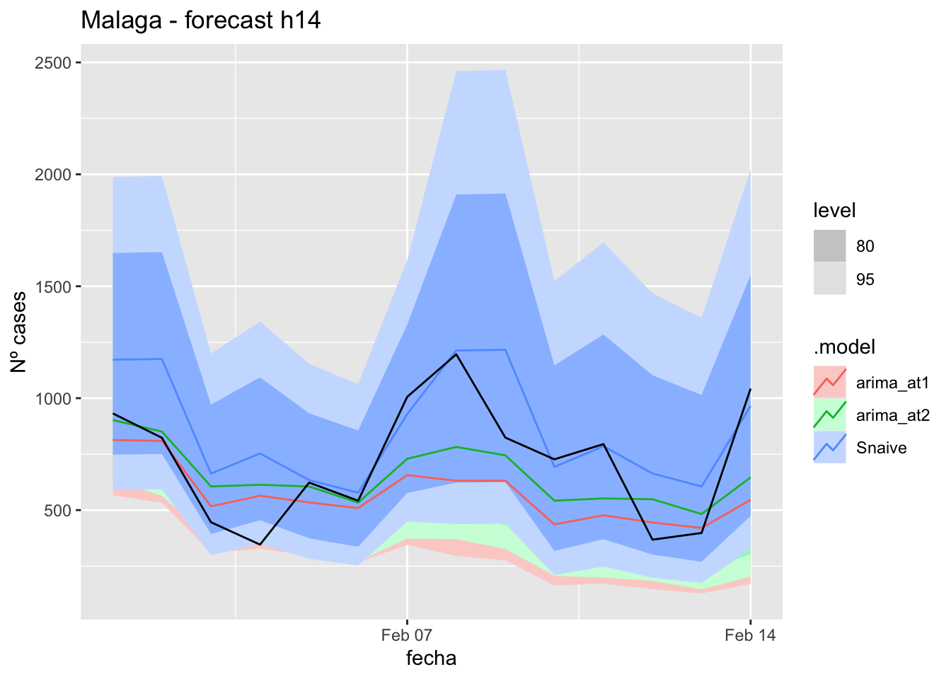
fc_h14 %>%
autoplot(
data_Malaga %>%
filter(fecha <= as.Date("2022-01-31", format = "%Y-%m-%d")+days(14) &
fecha > as.Date("2022-01-01", format = "%Y-%m-%d"))
) +
labs(y = "Nº cases", title = "Malaga - forecast h14")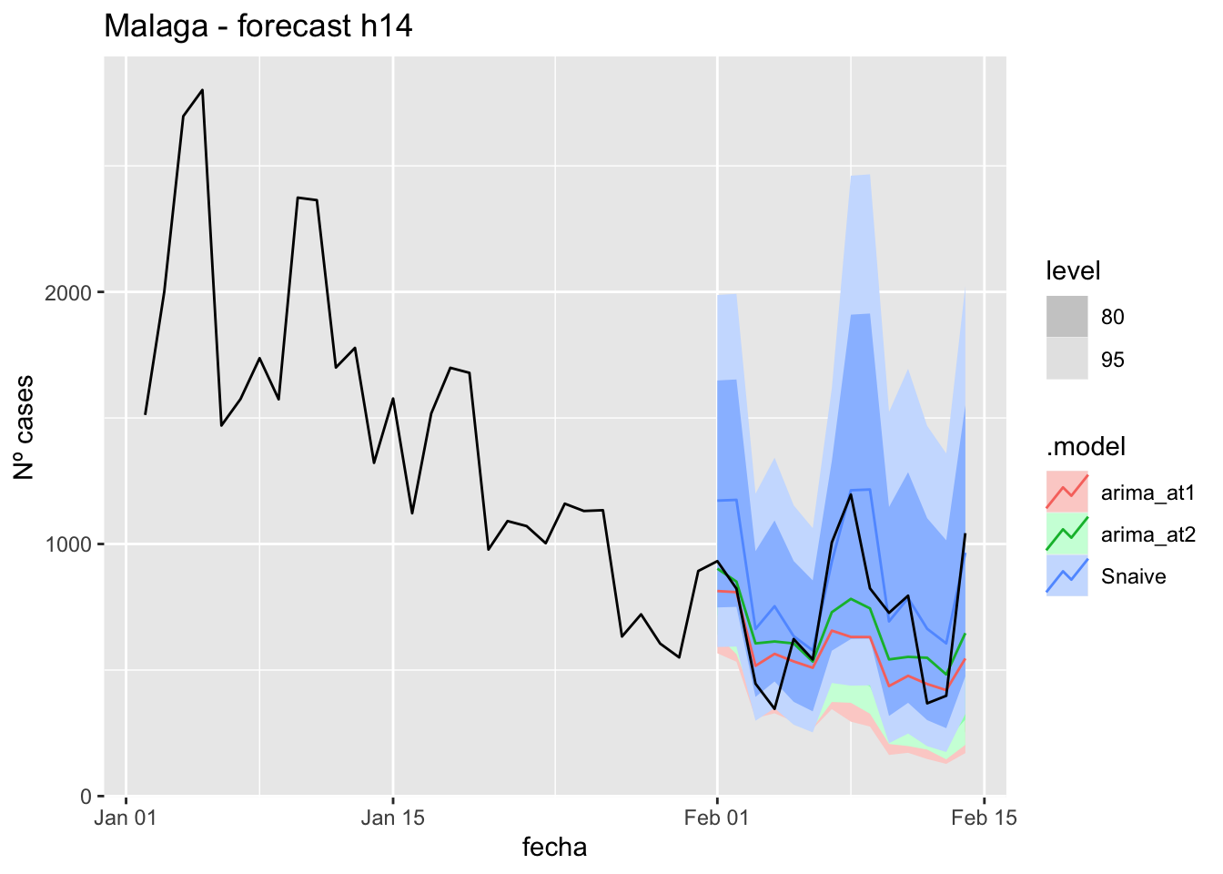
# Accuracy
fabletools::accuracy(fc_h14, data_Malaga)# A tibble: 3 × 11
.model provincia .type ME RMSE MAE MPE MAPE MASE RMSSE ACF1
<chr> <chr> <chr> <dbl> <dbl> <dbl> <dbl> <dbl> <dbl> <dbl> <dbl>
1 arima_at1 Málaga Test 149. 266. 204. 11.6 26.7 1.54 1.08 0.282
2 arima_at2 Málaga Test 66.4 214. 169. -0.972 25.7 1.28 0.866 0.260
3 Snaive Málaga Test -141. 223. 170. -28.9 31.8 1.28 0.899 0.023921 days
# Plots
fc_h21 %>%
autoplot(
data_Malaga_test %>%
filter(fecha <= as.Date("2022-01-31", format = "%Y-%m-%d")+days(21))
) +
labs(y = "Nº cases", title = "Malaga - forecast h21")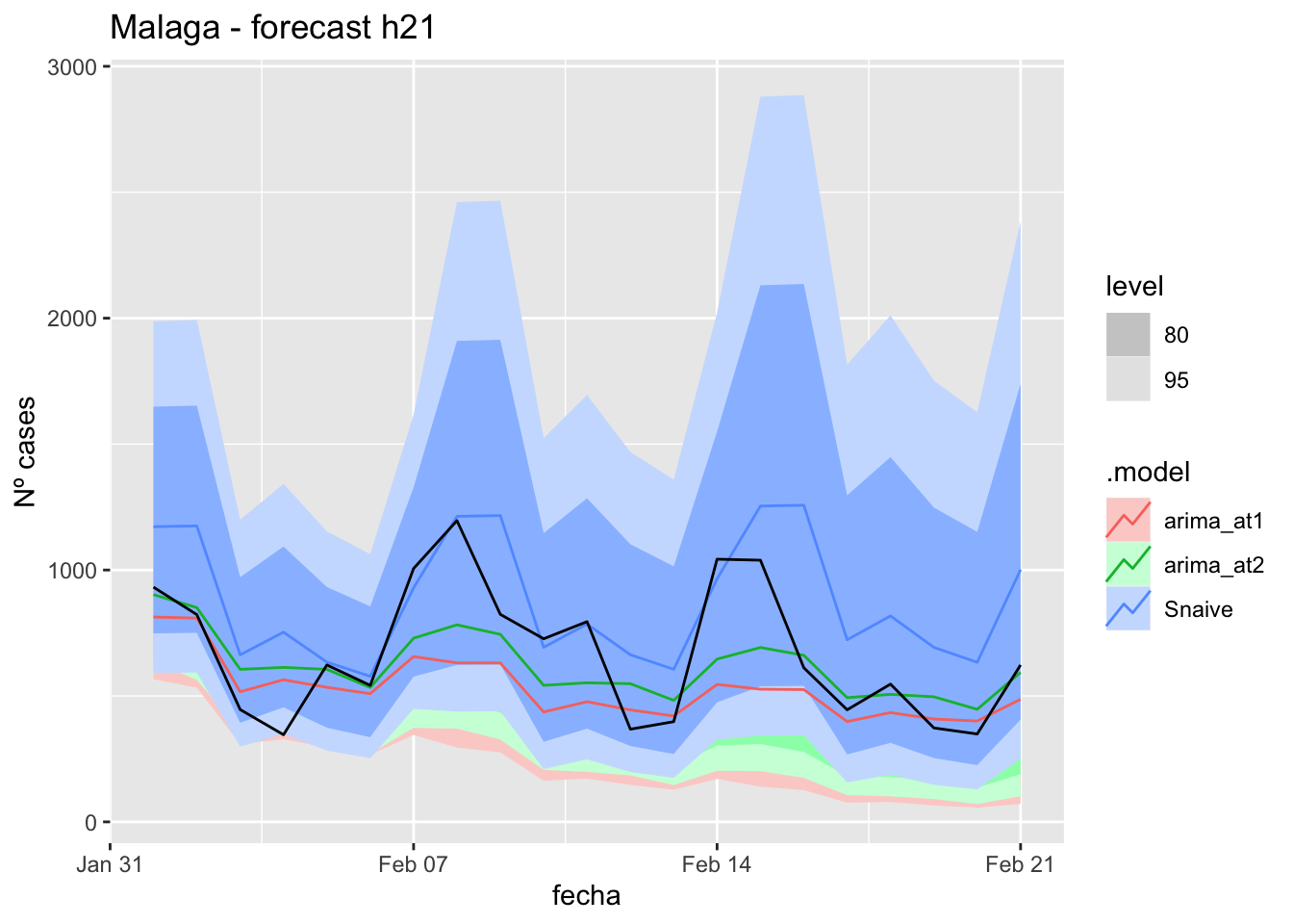
fc_h21 %>%
autoplot(
data_Malaga %>%
filter(fecha <= as.Date("2022-01-31", format = "%Y-%m-%d")+days(21) &
fecha > as.Date("2022-01-01", format = "%Y-%m-%d"))
) +
labs(y = "Nº cases", title = "Malaga - forecast h21")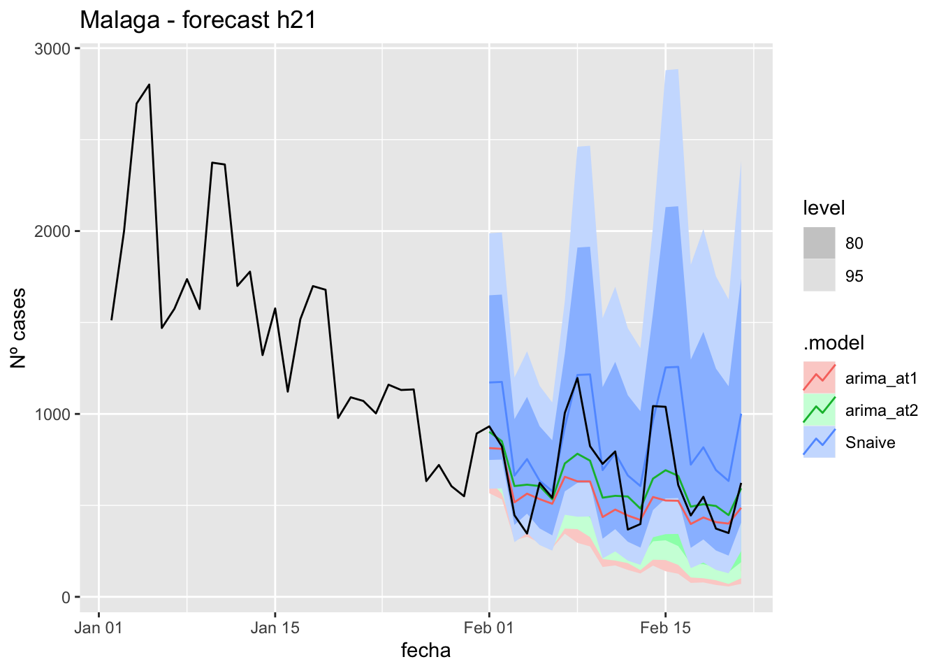
# Accuracy
fabletools::accuracy(fc_h21, data_Malaga)# A tibble: 3 × 11
.model provincia .type ME RMSE MAE MPE MAPE MASE RMSSE ACF1
<chr> <chr> <chr> <dbl> <dbl> <dbl> <dbl> <dbl> <dbl> <dbl> <dbl>
1 arima_at1 Málaga Test 137. 249. 183. 12.1 24.5 1.38 1.01 0.388
2 arima_at2 Málaga Test 48.9 195. 148. -2.29 23.1 1.12 0.786 0.354
3 Snaive Málaga Test -208. 279. 227. -41.4 43.4 1.72 1.13 0.17257 days
# Plots
fc_h57 %>%
autoplot(
data_Malaga_test %>%
filter(fecha <= as.Date("2022-01-31", format = "%Y-%m-%d")+days(57))
) +
labs(y = "Nº cases", title = "Malaga - forecast h57")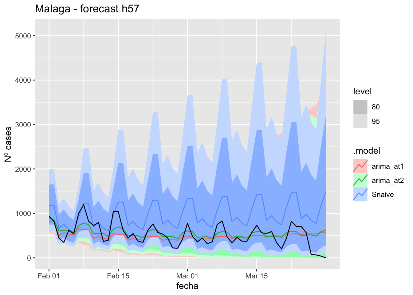
fc_h57 %>%
autoplot(
data_Malaga %>%
filter(fecha <= as.Date("2022-01-31", format = "%Y-%m-%d")+days(57) &
fecha > as.Date("2022-01-01", format = "%Y-%m-%d"))
) +
labs(y = "Nº cases", title = "Malaga - forecast h57")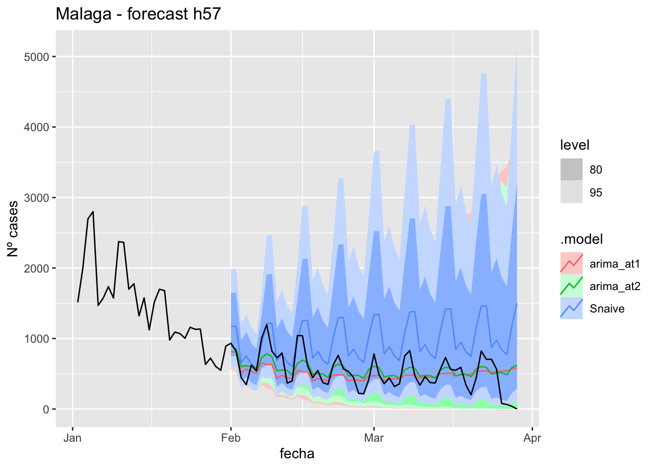
# Accuracy
fabletools::accuracy(fc_h57, data_Malaga)# A tibble: 3 × 11
.model provincia .type ME RMSE MAE MPE MAPE MASE RMSSE ACF1
<chr> <chr> <chr> <dbl> <dbl> <dbl> <dbl> <dbl> <dbl> <dbl> <dbl>
1 arima_at1 Málaga Test 36.7 237. 175. -Inf Inf 1.33 0.957 0.556
2 arima_at2 Málaga Test -24.7 208. 158. -Inf Inf 1.19 0.842 0.501
3 Snaive Málaga Test -436. 525. 443. -Inf Inf 3.35 2.12 0.513Sevilla
data_Sevilla <- covid_data %>%
filter(provincia == "Sevilla") %>%
filter(fecha > as.Date("2020-06-14", format = "%Y-%m-%d")) %>%
select(provincia, fecha, num_casos, tmed) %>%
drop_na() %>%
as_tsibble(key = provincia, index = fecha)
data_Sevilla# A tsibble: 653 x 4 [1D]
# Key: provincia [1]
provincia fecha num_casos tmed
<chr> <date> <dbl> <dbl>
1 Sevilla 2020-06-15 2 23.1
2 Sevilla 2020-06-16 1 24.0
3 Sevilla 2020-06-17 0 24.9
4 Sevilla 2020-06-18 0 25.8
5 Sevilla 2020-06-19 0 26.6
6 Sevilla 2020-06-20 0 27.5
7 Sevilla 2020-06-21 0 28.4
8 Sevilla 2020-06-22 1 29.3
9 Sevilla 2020-06-23 0 30.2
10 Sevilla 2020-06-24 1 29.4
# … with 643 more rowsdata_Sevilla_train <- data_Sevilla %>%
filter(fecha <= as.Date("2022-01-31", format = "%Y-%m-%d"))
summary(data_Sevilla_train$fecha) Min. 1st Qu. Median Mean 3rd Qu. Max.
"2020-06-15" "2020-11-10" "2021-04-08" "2021-04-08" "2021-09-04" "2022-01-31" data_Sevilla_test <- data_Sevilla %>%
filter(fecha > as.Date("2022-01-31", format = "%Y-%m-%d"))
summary(data_Sevilla_test$fecha) Min. 1st Qu. Median Mean 3rd Qu. Max.
"2022-02-01" "2022-02-15" "2022-03-01" "2022-03-01" "2022-03-15" "2022-03-29" # Lamba for num_casos
lambda_Sevilla_casos <- data_Sevilla %>%
features(num_casos, features = guerrero) %>%
pull(lambda_guerrero)
lambda_Sevilla_casos[1] 0.1933674# Lamba for average temp
lambda_Sevilla_tmed <- data_Sevilla %>%
features(tmed, features = guerrero) %>%
pull(lambda_guerrero)
lambda_Sevilla_tmed[1] 0.9333023fit_model <- data_Sevilla_train %>%
model(
arima_at1 = ARIMA(box_cox(num_casos, lambda_Sevilla_casos) ~
box_cox(tmed, lambda_Sevilla_tmed)),
arima_at2 = ARIMA(box_cox(num_casos, lambda_Sevilla_casos) ~
box_cox(tmed, lambda_Sevilla_tmed),
stepwise = FALSE, approx = FALSE),
Snaive = SNAIVE(box_cox(num_casos, lambda_Sevilla_casos))
)
# Show and report model
fit_model# A mable: 1 x 4
# Key: provincia [1]
provincia arima_at1
<chr> <model>
1 Sevilla <LM w/ ARIMA(3,1,1)(2,0,0)[7] errors>
# … with 2 more variables: arima_at2 <model>, Snaive <model>glance(fit_model)# A tibble: 3 × 9
provincia .model sigma2 log_lik AIC AICc BIC ar_roots ma_roots
<chr> <chr> <dbl> <dbl> <dbl> <dbl> <dbl> <list> <list>
1 Sevilla arima_at1 0.961 -832. 1679. 1679. 1714. <cpl [17]> <cpl [1]>
2 Sevilla arima_at2 0.961 -831. 1679. 1679. 1714. <cpl [18]> <cpl [0]>
3 Sevilla Snaive 2.23 NA NA NA NA <NULL> <NULL> fit_model %>%
pivot_longer(-provincia,
names_to = ".model",
values_to = "orders") %>%
left_join(glance(fit_model), by = c("provincia", ".model")) %>%
arrange(AICc) %>%
select(.model:BIC)# A mable: 3 x 7
# Key: .model [3]
.model orders sigma2 log_lik AIC AICc BIC
<chr> <model> <dbl> <dbl> <dbl> <dbl> <dbl>
1 arima_… <LM w/ ARIMA(4,1,0)(2,0,0)[7] errors> 0.961 -831. 1679. 1679. 1714.
2 arima_… <LM w/ ARIMA(3,1,1)(2,0,0)[7] errors> 0.961 -832. 1679. 1679. 1714.
3 Snaive <SNAIVE> 2.23 NA NA NA NA # We use a Ljung-Box test >> large p-value, confirms residuals are similar / considered to white noise
fit_model %>%
select(Snaive) %>%
gg_tsresiduals()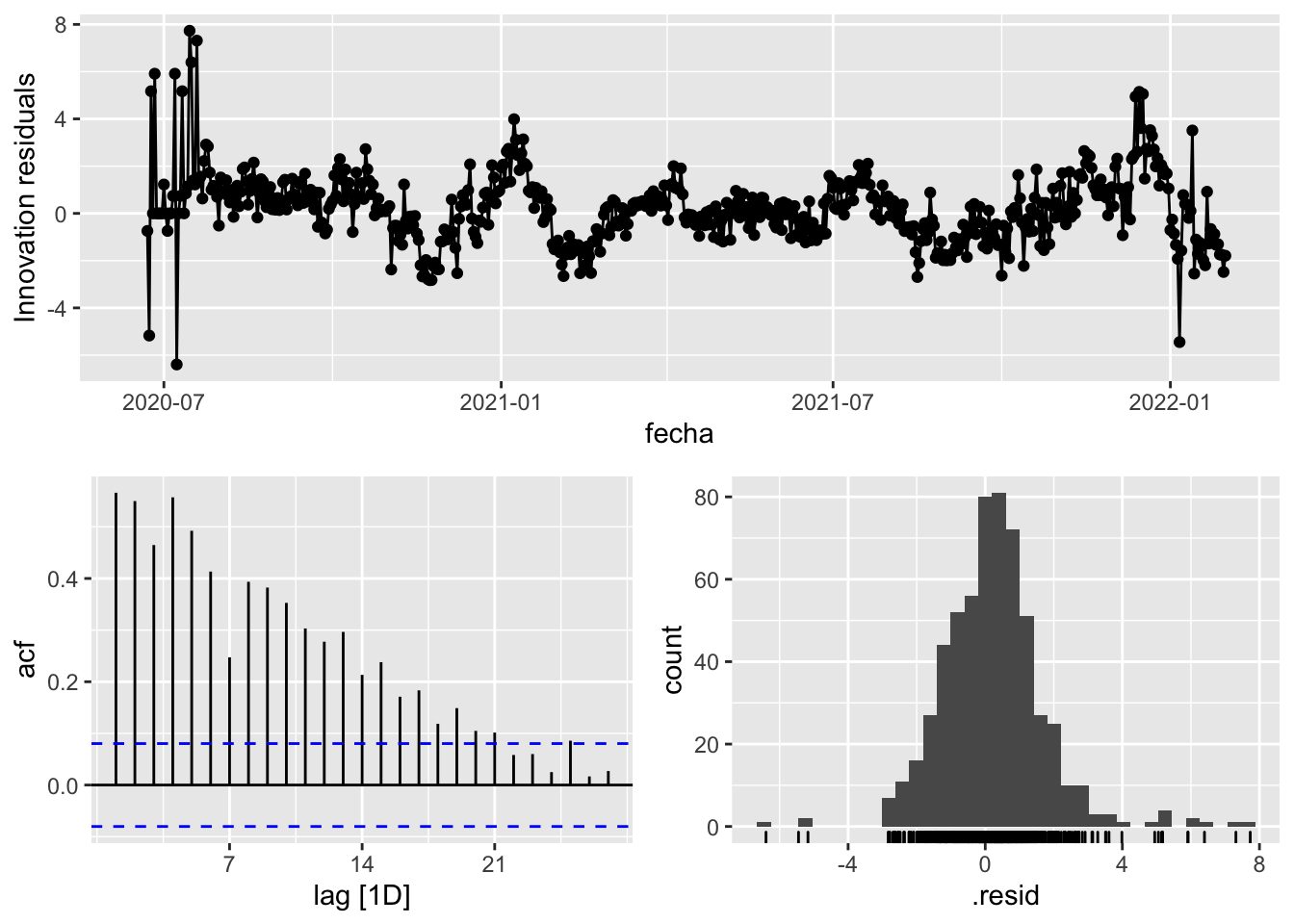
fit_model %>%
select(arima_at1) %>%
gg_tsresiduals()
fit_model %>%
select(arima_at2) %>%
gg_tsresiduals()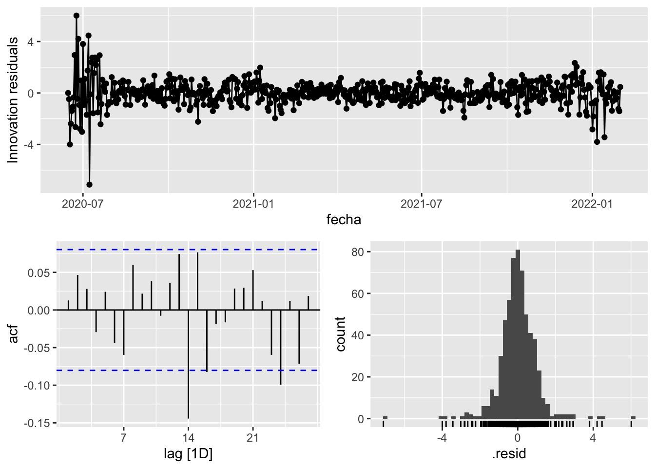
augment(fit_model) %>%
features(.innov, ljung_box, lag=7)# A tibble: 3 × 4
provincia .model lb_stat lb_pvalue
<chr> <chr> <dbl> <dbl>
1 Sevilla arima_at1 6.88 0.441
2 Sevilla arima_at2 6.06 0.533
3 Sevilla Snaive 965. 0 augment(fit_model) %>%
features(.innov, ljung_box, lag=14)# A tibble: 3 × 4
provincia .model lb_stat lb_pvalue
<chr> <chr> <dbl> <dbl>
1 Sevilla arima_at1 27.0 0.0190
2 Sevilla arima_at2 26.4 0.0232
3 Sevilla Snaive 1403. 0 augment(fit_model) %>%
features(.innov, ljung_box, lag=21)# A tibble: 3 × 4
provincia .model lb_stat lb_pvalue
<chr> <chr> <dbl> <dbl>
1 Sevilla arima_at1 37.9 0.0132
2 Sevilla arima_at2 37.3 0.0155
3 Sevilla Snaive 1510. 0 augment(fit_model) %>%
features(.innov, ljung_box, lag=57)# A tibble: 3 × 4
provincia .model lb_stat lb_pvalue
<chr> <chr> <dbl> <dbl>
1 Sevilla arima_at1 76.9 0.0406
2 Sevilla arima_at2 76.4 0.0439
3 Sevilla Snaive 1813. 0 # To predict future values of infections, we need to pass the model future/prediction values of the complementary variables tmed and mobility
# We are going to select those from the test dataset
data_fc_h7 <- data_Sevilla_test %>%
select(-num_casos) %>%
slice(1:7)
data_fc_h14 <- data_Sevilla_test %>%
select(-num_casos) %>%
slice(1:14)
data_fc_h21 <- data_Sevilla_test %>%
select(-num_casos) %>%
slice(1:21)
data_fc_h57 <- data_Sevilla_test %>%
select(-num_casos) %>%
slice(1:57)# Significant spikes out of 30 is still consistent with white noise
# To be sure, use a Ljung-Box test, which has a large p-value, confirming that
# the residuals are similar to white noise.
# Note that the alternative models also passed this test.
#
# Forecast
fc_h7 <- fabletools::forecast(fit_model, new_data = data_fc_h7)
fc_h14 <- fabletools::forecast(fit_model, new_data = data_fc_h14)
fc_h21 <- fabletools::forecast(fit_model, new_data = data_fc_h21)
fc_h57 <- fabletools::forecast(fit_model, new_data = data_fc_h57)7 days
# Plots
fc_h7 %>%
autoplot(
data_Sevilla_test %>%
filter(fecha <= as.Date("2022-01-31", format = "%Y-%m-%d")+days(7))
) +
labs(y = "Nº cases", title = "Sevilla - forecast h7")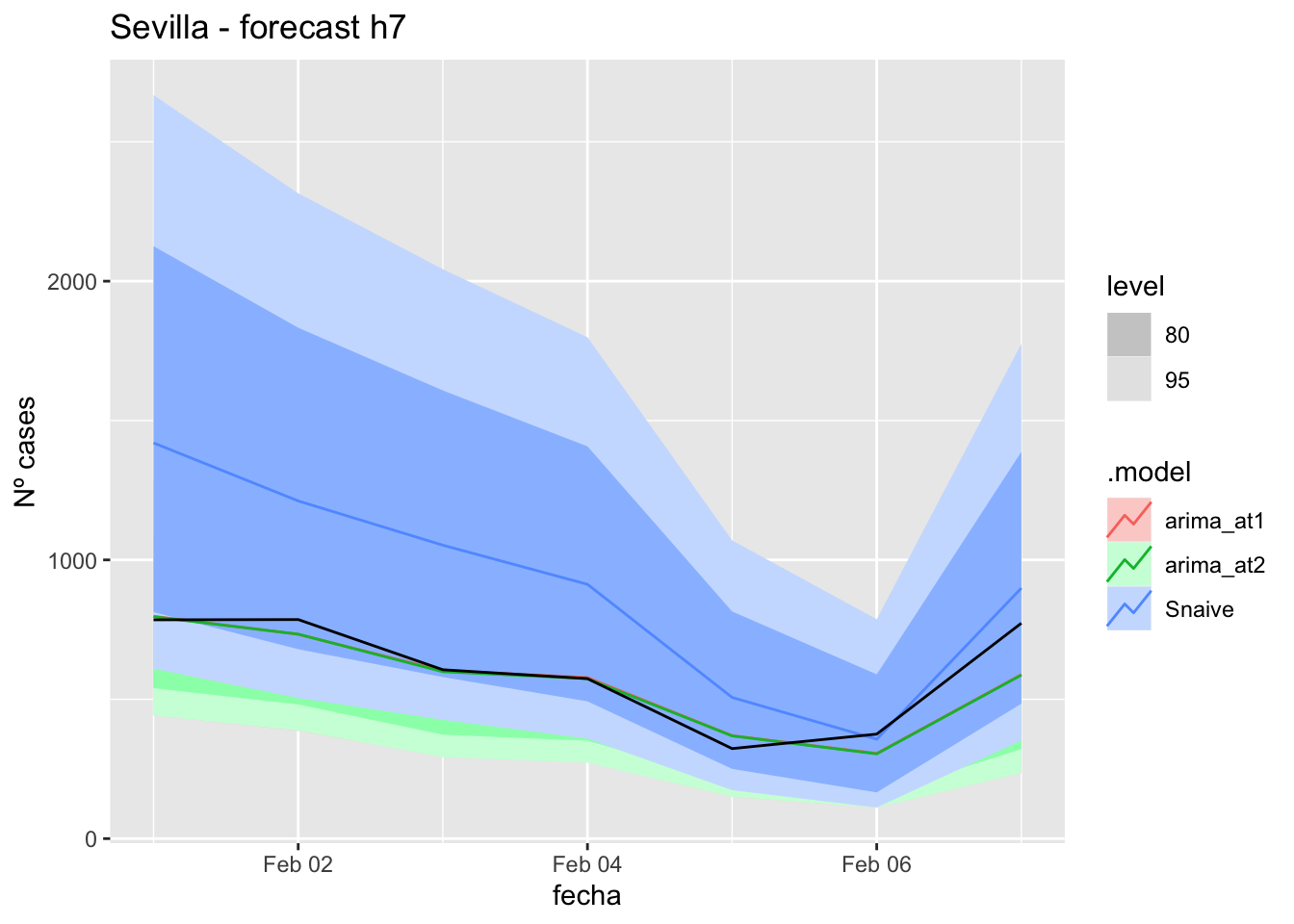
fc_h7 %>%
autoplot(
data_Sevilla %>%
filter(fecha <= as.Date("2022-01-31", format = "%Y-%m-%d")+days(7) &
fecha > as.Date("2022-01-01", format = "%Y-%m-%d"))
) +
labs(y = "Nº cases", title = "Sevilla - forecast h7")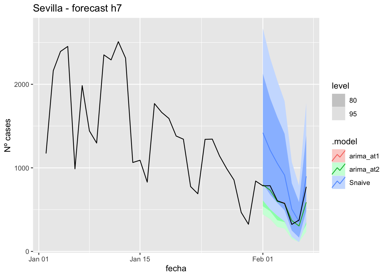
# Accuracy
fabletools::accuracy(fc_h7, data_Sevilla)# A tibble: 3 × 11
.model provincia .type ME RMSE MAE MPE MAPE MASE RMSSE ACF1
<chr> <chr> <chr> <dbl> <dbl> <dbl> <dbl> <dbl> <dbl> <dbl> <dbl>
1 arima_at1 Sevilla Test 35.3 79.3 53.4 4.72 9.49 0.373 0.291 0.152
2 arima_at2 Sevilla Test 37.0 79.8 53.3 5.02 9.48 0.372 0.292 0.149
3 Snaive Sevilla Test -305. 368. 311. -48.0 49.4 2.17 1.35 0.52314 days
# Plots
fc_h14 %>%
autoplot(
data_Sevilla_test %>%
filter(fecha <= as.Date("2022-01-31", format = "%Y-%m-%d")+days(14))
) +
labs(y = "Nº cases", title = "Sevilla - forecast h14")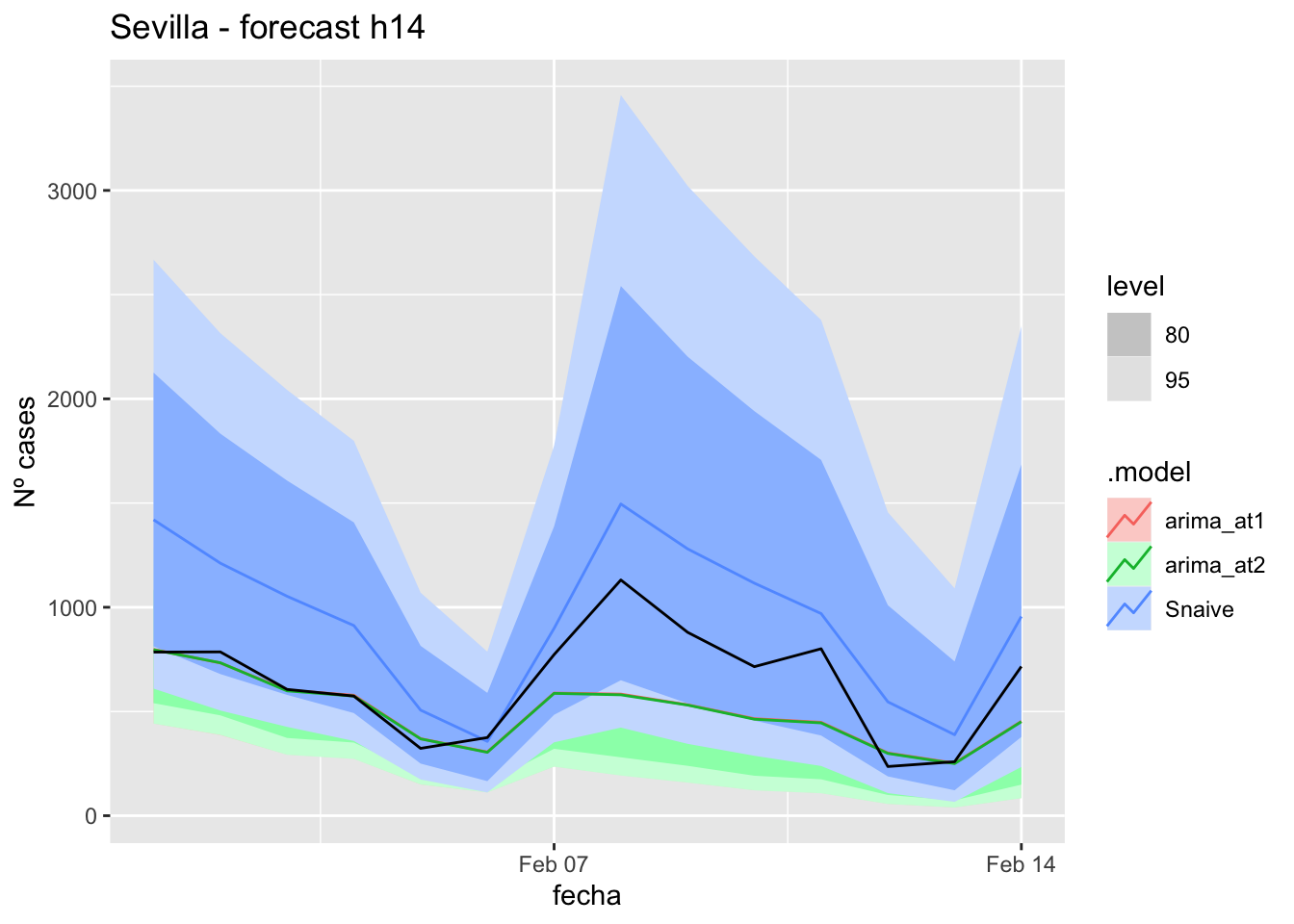
fc_h14 %>%
autoplot(
data_Sevilla %>%
filter(fecha <= as.Date("2022-01-31", format = "%Y-%m-%d")+days(14) &
fecha > as.Date("2022-01-01", format = "%Y-%m-%d"))
) +
labs(y = "Nº cases", title = "Sevilla - forecast h14")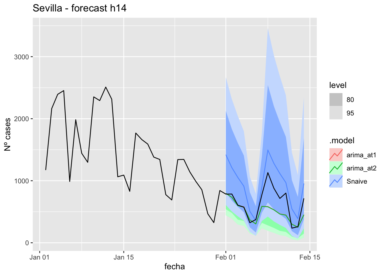
# Accuracy
fabletools::accuracy(fc_h14, data_Sevilla)# A tibble: 3 × 11
.model provincia .type ME RMSE MAE MPE MAPE MASE RMSSE ACF1
<chr> <chr> <chr> <dbl> <dbl> <dbl> <dbl> <dbl> <dbl> <dbl> <dbl>
1 arima_at1 Sevilla Test 139. 228. 158. 15.1 21.4 1.10 0.834 0.436
2 arima_at2 Sevilla Test 141. 229. 158. 15.5 21.5 1.11 0.839 0.435
3 Snaive Sevilla Test -297. 338. 299. -50.4 51.1 2.09 1.24 0.41121 days
# Plots
fc_h21 %>%
autoplot(
data_Sevilla_test %>%
filter(fecha <= as.Date("2022-01-31", format = "%Y-%m-%d")+days(21))
) +
labs(y = "Nº cases", title = "Sevilla - forecast h21")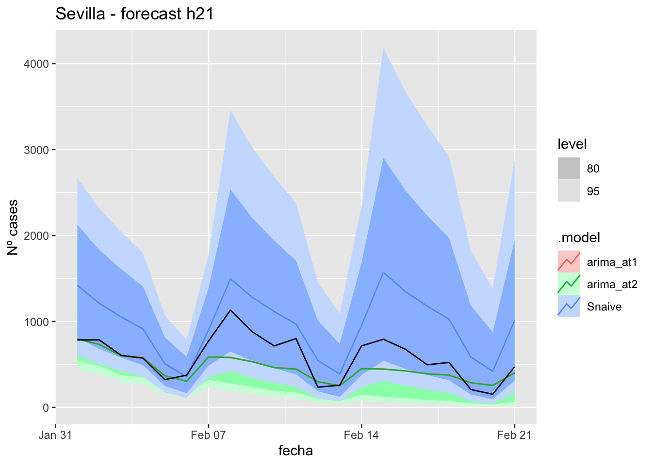
fc_h21 %>%
autoplot(
data_Sevilla %>%
filter(fecha <= as.Date("2022-01-31", format = "%Y-%m-%d")+days(21) &
fecha > as.Date("2022-01-01", format = "%Y-%m-%d"))
) +
labs(y = "Nº cases", title = "Sevilla - forecast h21")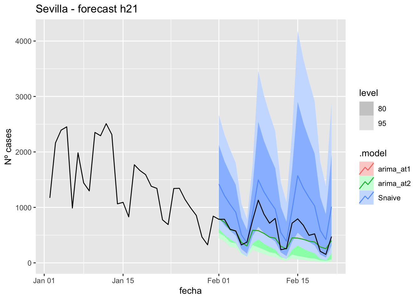
# Accuracy
fabletools::accuracy(fc_h21, data_Sevilla)# A tibble: 3 × 11
.model provincia .type ME RMSE MAE MPE MAPE MASE RMSSE ACF1
<chr> <chr> <chr> <dbl> <dbl> <dbl> <dbl> <dbl> <dbl> <dbl> <dbl>
1 arima_at1 Sevilla Test 128. 214. 157. 11.9 26.2 1.10 0.784 0.502
2 arima_at2 Sevilla Test 130. 215. 158. 12.3 26.3 1.11 0.789 0.501
3 Snaive Sevilla Test -380. 430. 381. -76.5 77.0 2.67 1.58 0.50757 days
# Plots
fc_h57 %>%
autoplot(
data_Sevilla_test %>%
filter(fecha <= as.Date("2022-01-31", format = "%Y-%m-%d")+days(57))
) +
labs(y = "Nº cases", title = "Sevilla - forecast h57")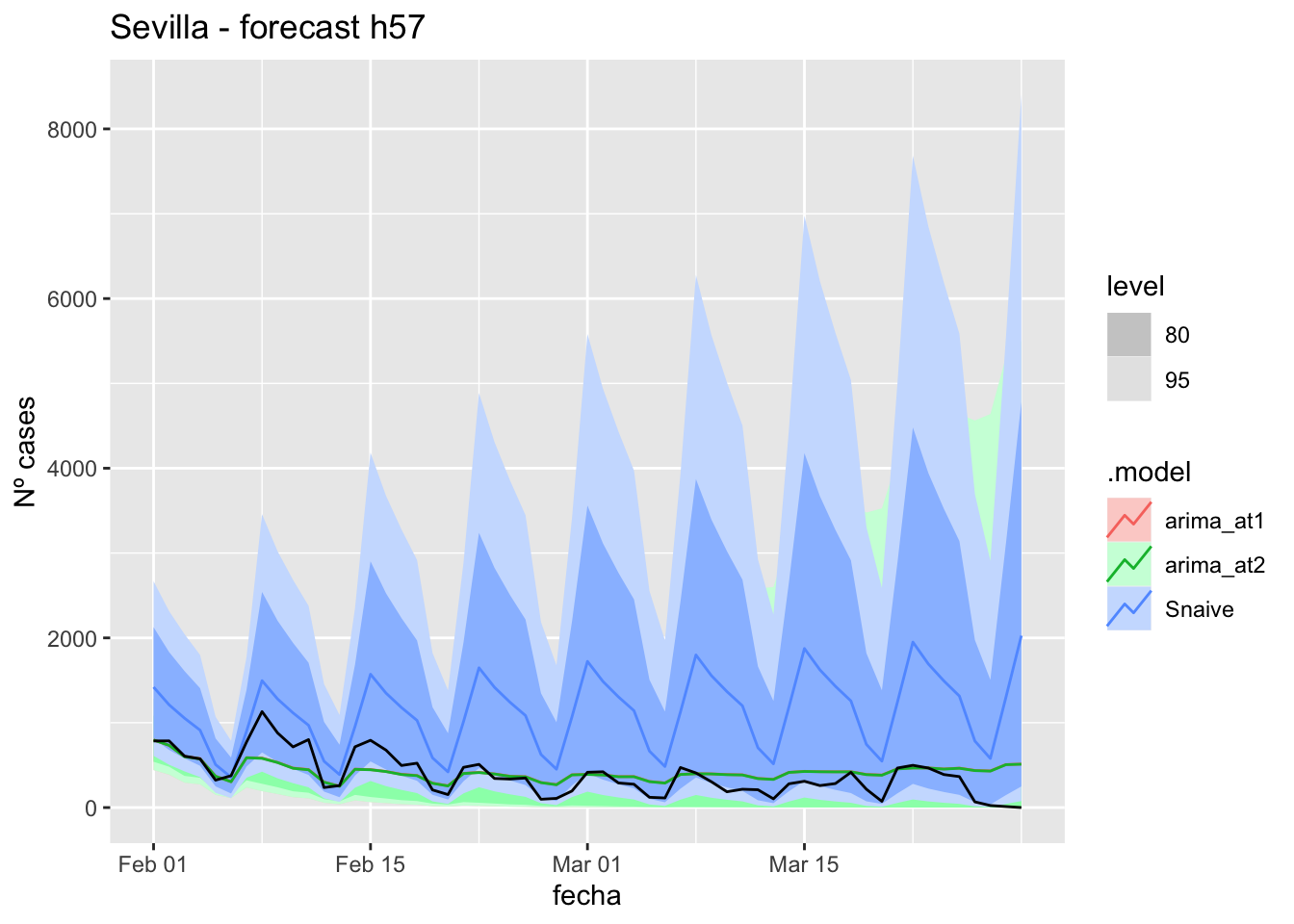
fc_h57 %>%
autoplot(
data_Sevilla %>%
filter(fecha <= as.Date("2022-01-31", format = "%Y-%m-%d")+days(57) &
fecha > as.Date("2022-01-01", format = "%Y-%m-%d"))
) +
labs(y = "Nº cases", title = "Sevilla - forecast h57")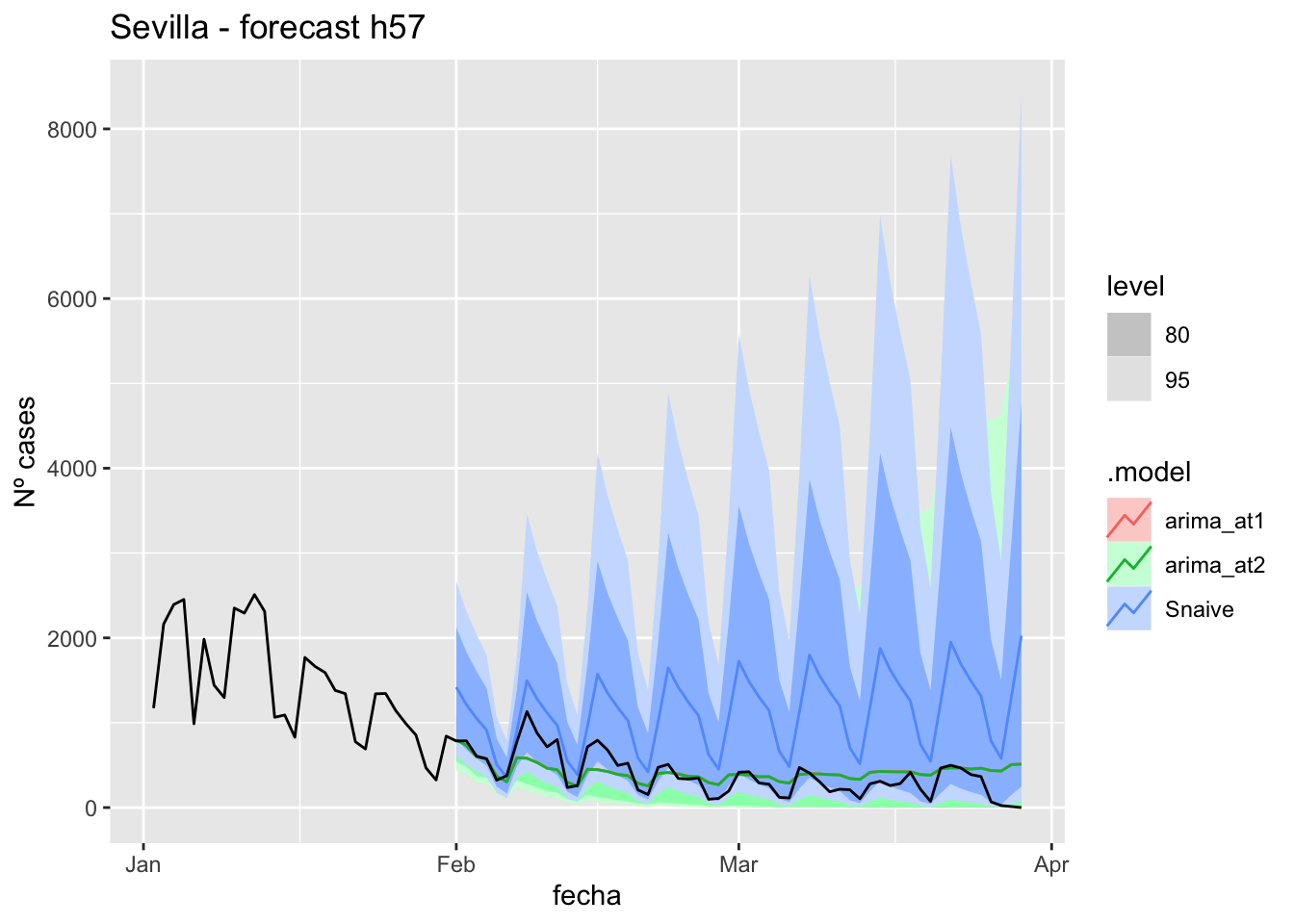
# Accuracy
fabletools::accuracy(fc_h57, data_Sevilla)# A tibble: 3 × 11
.model provincia .type ME RMSE MAE MPE MAPE MASE RMSSE ACF1
<chr> <chr> <chr> <dbl> <dbl> <dbl> <dbl> <dbl> <dbl> <dbl> <dbl>
1 arima_at1 Sevilla Test -36.1 203. 151. -Inf Inf 1.06 0.744 0.710
2 arima_at2 Sevilla Test -34.1 203. 151. -Inf Inf 1.05 0.743 0.709
3 Snaive Sevilla Test -737. 850. 738. -Inf Inf 5.16 3.11 0.642