LSTM multivariate prediction

Import python packages:

import numpy as np
import pandas as pd
import matplotlib
import matplotlib.pyplot as plt

from sklearn.preprocessing import MinMaxScaler
from sklearn.metrics import mean_absolute_error, mean_squared_error

from keras import Input
from keras.models import Sequential
from keras.layers import Dense, LSTM
from keras.layers.core import Dense, Activation, Dropout

data_covid = pd.read_csv('data/clean/final_covid_data.csv')
data_covid

	provincia	fecha	num_casos	num_casos_prueba_pcr	num_casos_prueba_test_ac	num_casos_prueba_ag	num_casos_prueba_elisa	num_casos_prueba_desconocida	num_hosp	num_uci	...	ws	ws_max	sol	mob_grocery_pharmacy	mob_parks	mob_residential	mob_retail_recreation	mob_transit_stations	mob_workplaces	mob_flujo
0	Barcelona	2020-01-01	0	0	0	0	0	0	0	0	...	2.5	7.2	4.9	NaN	NaN	NaN	NaN	NaN	NaN	NaN
1	Madrid	2020-01-01	1	1	0	0	0	0	1	0	...	0.8	3.6	8.3	NaN	NaN	NaN	NaN	NaN	NaN	NaN
2	Málaga	2020-01-01	0	0	0	0	0	0	0	0	...	3.3	6.7	7.7	NaN	NaN	NaN	NaN	NaN	NaN	NaN
3	Asturias	2020-01-01	0	0	0	0	0	0	0	0	...	2.5	7.8	7.9	NaN	NaN	NaN	NaN	NaN	NaN	NaN
4	Sevilla	2020-01-01	0	0	0	0	0	0	1	0	...	1.9	5.8	9.1	NaN	NaN	NaN	NaN	NaN	NaN	NaN
...	...	...	...	...	...	...	...	...	...	...	...	...	...	...	...	...	...	...	...	...	...
4090	Barcelona	2022-03-29	0	0	0	0	0	0	0	0	...	7.2	13.3	0.0	0.0	-13.0	5.0	-24.0	-16.0	-17.0	NaN
4091	Madrid	2022-03-29	6	3	0	3	0	0	0	0	...	2.2	6.1	2.4	1.0	-11.0	4.0	-25.0	-16.0	-16.0	NaN
4092	Málaga	2022-03-29	0	0	0	0	0	0	0	0	...	4.2	10.8	1.5	4.0	-3.0	4.0	-16.0	1.0	-8.0	NaN
4093	Asturias	2022-03-29	0	0	0	0	0	0	1	0	...	2.2	6.7	0.0	-4.0	17.0	3.0	-25.0	-15.0	-12.0	NaN
4094	Sevilla	2022-03-29	0	0	0	0	0	0	0	0	...	2.5	8.3	1.6	3.0	-7.0	2.0	-15.0	-13.0	-5.0	NaN

4095 rows × 26 columns

All the available data

Asturias

data_asturias = data_covid.loc[data_covid['provincia'] == 'Asturias']
data_asturias = data_asturias.set_index('fecha')
data_asturias = data_asturias['2020-06-14':]
data_asturias = data_asturias.filter(['num_casos', 'tmed', 'mob_grocery_pharmacy', 
'mob_parks', 'mob_residential', 'mob_residential', 'mob_transit_stations', 'mob_workplaces'])
data_asturias

	num_casos	tmed	mob_grocery_pharmacy	mob_parks	mob_residential	mob_residential	mob_transit_stations	mob_workplaces
fecha
2020-06-14	0	16.8	-8.0	6.0	4.0	4.0	-43.0	-2.0
2020-06-15	0	16.0	-6.0	39.0	7.0	7.0	-38.0	-27.0
2020-06-16	1	15.6	-6.0	7.0	9.0	9.0	-43.0	-29.0
2020-06-17	0	15.6	-7.0	20.0	8.0	8.0	-42.0	-28.0
2020-06-18	0	15.1	-4.0	68.0	7.0	7.0	-39.0	-28.0
...	...	...	...	...	...	...	...	...
2022-03-25	244	11.6	-2.0	24.0	2.0	2.0	-13.0	-12.0
2022-03-26	432	12.0	-13.0	27.0	1.0	1.0	-19.0	-13.0
2022-03-27	1	14.2	-7.5	33.0	-1.0	-1.0	-13.0	-11.0
2022-03-28	9	13.8	-2.0	45.0	1.0	1.0	-9.0	-10.0
2022-03-29	0	11.7	-4.0	17.0	3.0	3.0	-15.0	-12.0

654 rows × 8 columns

data_asturias.describe()

	num_casos	tmed	mob_grocery_pharmacy	mob_parks	mob_residential	mob_residential	mob_transit_stations	mob_workplaces
count	654.00000	654.000000	654.00000	654.000000	654.000000	654.000000	654.000000	654.000000
mean	312.11315	13.909098	3.83792	57.725535	3.695719	3.695719	-12.614679	-20.651376
std	565.17985	4.198047	15.05797	68.024228	4.802763	4.802763	14.838430	12.754756
min	0.00000	3.300000	-87.00000	-63.000000	-8.000000	-8.000000	-67.000000	-80.000000
25%	43.50000	10.800000	-0.50000	13.000000	1.000000	1.000000	-22.000000	-26.000000
50%	117.00000	13.900000	5.00000	39.000000	3.000000	3.000000	-13.000000	-18.500000
75%	323.75000	17.600000	10.00000	83.500000	6.000000	6.000000	-4.000000	-14.000000
max	3827.00000	25.100000	42.00000	333.000000	26.000000	26.000000	26.000000	12.000000

np_data_asturias = data_asturias.values

# Train dataset
scaler = MinMaxScaler(feature_range=(0, 1))
scaled_data_asturias = scaler.fit_transform(np_data_asturias)
print(f'Longitud del conjunto de datos disponible: {len(scaled_data_asturias)}')

Longitud del conjunto de datos disponible: 654

# Since we are going to predict future values based on the 90 past elements, 
# we need to create a list with those historic information for each element
historic_values = 90
scaled_data_asturias_x = []
scaled_data_asturias_y = []

for i in range(historic_values, len(scaled_data_asturias)):
    scaled_data_asturias_x.append(scaled_data_asturias[(i-historic_values):i, :])
    scaled_data_asturias_y.append(scaled_data_asturias[i, 0])

# Convert the x_train and y_train to numpy arrays
scaled_data_asturias_x = np.array(scaled_data_asturias_x)
scaled_data_asturias_y = np.array(scaled_data_asturias_y)

# Once predicted, we are going to need a exclusive scaler for num_cases
scaler_pred = MinMaxScaler(feature_range=(0, 1))
df_cases_asturias = pd.DataFrame(data_asturias['num_casos'])
scaled_data_asturias_pred = scaler_pred.fit_transform(df_cases_asturias)

# Since the first 90th values does not have historic, the dataset has been reduced in 90 values
print(f'Longitud datos de entrenamiento con historico: {len(scaled_data_asturias_y)}')

Longitud datos de entrenamiento con historico: 564

# we split data in train and test
# as in previous analysis, we are going to predict a maximum of 90 days
x_train = scaled_data_asturias_x[0:len(scaled_data_asturias_x)-91]
y_train = scaled_data_asturias_y[0:len(scaled_data_asturias_y)-91]
print(f'Cantidad datos de entrenamiento: x={len(x_train)} - y={len(y_train)}')

x_test = scaled_data_asturias_x[len(scaled_data_asturias_x)-90:len(scaled_data_asturias_x)]
y_test = scaled_data_asturias_y[len(scaled_data_asturias_y)-90:len(scaled_data_asturias_y)]
print(f'Cantidad datos de test: x={len(x_test)} - y={len(y_test)}')

Cantidad datos de entrenamiento: x=473 - y=473
Cantidad datos de test: x=90 - y=90

# Reshape the data to feed de recurrent network
x_train = np.reshape(x_train, (x_train.shape[0], x_train.shape[1], 8))
print("Train data shape:")
print(x_train.shape)
print(y_train.shape)
x_test = np.reshape(x_test, (x_test.shape[0], x_test.shape[1], 8))
print("Test data shape:")
print(x_test.shape)
print(y_test.shape)

Train data shape:
(473, 90, 8)
(473,)
Test data shape:
(90, 90, 8)
(90,)

# Configure / setup the neural network model - LSTM
# Build the model
print('Build model...')
model = Sequential()
# Model with Neurons 
# Inputshape = neurons -> Timestamps
neurons= x_train.shape[1]
model.add(LSTM(90, 
               activation = 'relu',
               return_sequences = True, 
               input_shape = (x_train.shape[1], 8))) 
model.add(LSTM(50, 
               activation = 'relu',
               return_sequences = True)) 
model.add(LSTM(25, 
               activation = 'relu',
               return_sequences = False)) 
model.add(Dense(5, activation = 'relu'))
model.add(Dense(1))

Build model...

2022-05-25 01:28:48.052818: I tensorflow/core/platform/cpu_feature_guard.cc:193] This TensorFlow binary is optimized with oneAPI Deep Neural Network Library (oneDNN) to use the following CPU instructions in performance-critical operations:  AVX2 FMA
To enable them in other operations, rebuild TensorFlow with the appropriate compiler flags.

model.compile(optimizer='adam', loss='mean_squared_error')
model.summary()

Model: "sequential"

_________________________________________________________________

 Layer (type)                Output Shape              Param #   

=================================================================

 lstm (LSTM)                 (None, 90, 90)            35640     

 lstm_1 (LSTM)               (None, 90, 50)            28200     

 lstm_2 (LSTM)               (None, 25)                7600      

 dense (Dense)               (None, 5)                 130       

 dense_1 (Dense)             (None, 1)                 6         

=================================================================

Total params: 71,576

Trainable params: 71,576

Non-trainable params: 0

_________________________________________________________________

# Training the model
# fit network
history = model.fit(x_train, 
                    y_train, 
                    batch_size=1000, 
                    epochs=30, 
                    validation_data = (x_test, y_test), 
                    verbose = 0)

plt.plot(history.history['loss'], label='train')
plt.plot(history.history['val_loss'], label='test')
plt.legend()
plt.show()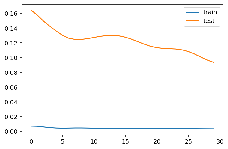 

# Get the predicted values
predictions = model.predict(x_test)
predictions = scaler_pred.inverse_transform(predictions)

1/3 [=========>....................] - ETA: 0s

3/3 [==============================] - ETA: 0s

3/3 [==============================] - 0s 30ms/step

y_test = y_test.reshape(-1,1)
y_test = scaler_pred.inverse_transform(y_test)

# Calculate the mean absolute error (MAE)
mae = mean_absolute_error(y_test, predictions)
print('MAE: ' + str(round(mae, 1)))

# Calculate the root mean squarred error (RMSE)
rmse = np.sqrt(mean_squared_error(y_test,predictions))
print('RMSE: ' + str(round(rmse, 1)))

# Calculate the root mean squarred error (RMSE)
rmse = mean_squared_error(y_test, 
                          predictions,
                          squared = False)
print('RMSE: ' + str(round(rmse, 1)))

MAE: 738.5
RMSE: 1169.8
RMSE: 1169.8

# Add the difference between the valid and predicted prices
train = data_asturias[:(len(x_train)+92)]
valid = data_asturias[(len(x_train)+91):]

valid.insert(1, "Predictions", predictions, True)
valid.insert(1, "Difference", valid["Predictions"] - valid["num_casos"], True)

# Zoom-in to a closer timeframe
# Date from which on the date is displayed
display_start_date = "2021-10-31" 
valid = valid[valid.index > display_start_date]
train = train[train.index > display_start_date]

# Visualize the data
matplotlib.style.use('ggplot')
fig, ax1 = plt.subplots(figsize=(22, 10), sharex=True)

# Data - Train
xt = train.index; 
yt = train[["num_casos"]]
# Data - Test / validation 
xv = valid.index; 
yv = valid[["num_casos", "Predictions"]]

# Plot
plt.title("Asturias: Predictions vs Real infections", fontsize=20)
plt.ylabel("Nº Cases", fontsize=18)

plt.plot(yt, color="blue", linewidth=1.5)
plt.plot(yv["Predictions"], color="red", linewidth=1.5)
plt.plot(yv["num_casos"], color="green", linewidth=1.5)
plt.legend(["Train", "LSTM Predictions", "Test"], 
           loc="upper left", fontsize=18)

# Bar plot with the differences
x = valid.index
y = valid["Difference"]
plt.bar(x, y, width=0.2, color="grey")
plt.grid()
plt.show()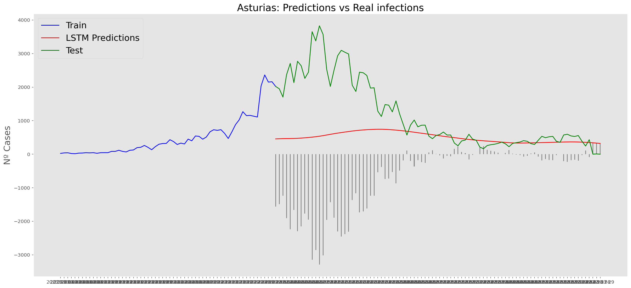

Barcelona

data_barcelona = data_covid.loc[data_covid['provincia'] == 'Barcelona']
data_barcelona = data_barcelona.set_index('fecha')
data_barcelona = data_barcelona['2020-06-14':]
data_barcelona = data_barcelona.filter(['num_casos', 'tmed', 'mob_grocery_pharmacy', 
'mob_parks', 'mob_residential', 'mob_residential', 'mob_transit_stations', 'mob_workplaces'])
data_barcelona

	num_casos	tmed	mob_grocery_pharmacy	mob_parks	mob_residential	mob_residential	mob_transit_stations	mob_workplaces
fecha
2020-06-14	33	20.6	-20.0	15.0	6.0	6.0	-31.0	-6.0
2020-06-15	62	21.2	-9.0	17.0	14.0	14.0	-34.0	-41.0
2020-06-16	66	20.8	-10.0	-16.0	16.0	16.0	-39.0	-41.0
2020-06-17	70	20.3	-4.0	14.0	15.0	15.0	-33.0	-40.0
2020-06-18	68	18.8	-8.0	-6.0	16.0	16.0	-38.0	-41.0
...	...	...	...	...	...	...	...	...
2022-03-25	598	14.4	3.0	-11.0	4.0	4.0	-18.0	-16.0
2022-03-26	345	12.8	-11.0	-33.0	3.0	3.0	-22.0	-12.0
2022-03-27	252	15.6	-10.0	-3.0	0.0	0.0	-12.0	-10.0
2022-03-28	688	14.0	-1.0	-2.0	4.0	4.0	-15.0	-15.0
2022-03-29	0	13.0	0.0	-13.0	5.0	5.0	-16.0	-17.0

654 rows × 8 columns

data_barcelona.describe()

	num_casos	tmed	mob_grocery_pharmacy	mob_parks	mob_residential	mob_residential	mob_transit_stations	mob_workplaces
count	654.000000	654.000000	654.000000	654.000000	654.000000	654.000000	654.000000	654.000000
mean	2605.048930	17.294801	0.180428	-5.547401	7.178899	7.178899	-24.041284	-27.391437
std	4823.001644	6.163636	16.568328	15.365483	5.019727	5.019727	11.241460	15.949374
min	0.000000	4.300000	-83.000000	-76.000000	-6.000000	-6.000000	-72.000000	-87.000000
25%	597.250000	12.200000	-7.000000	-15.000000	4.000000	4.000000	-32.000000	-34.000000
50%	1030.500000	16.300000	2.000000	-5.000000	7.000000	7.000000	-24.000000	-25.000000
75%	2243.750000	23.600000	10.000000	6.000000	10.000000	10.000000	-15.000000	-18.000000
max	34701.000000	28.400000	58.000000	33.000000	32.000000	32.000000	-2.000000	6.000000

np_data_barcelona = data_barcelona.values

# Train dataset
scaler = MinMaxScaler(feature_range=(0, 1))
scaled_data_barcelona = scaler.fit_transform(np_data_barcelona)
print(f'Longitud del conjunto de datos disponible: {len(scaled_data_barcelona)}')

Longitud del conjunto de datos disponible: 654

# Since we are going to predict future values based on the 90 past elements, 
# we need to create a list with those historic information for each element
historic_values = 90
scaled_data_barcelona_x = []
scaled_data_barcelona_y = []

for i in range(historic_values, len(scaled_data_barcelona)):
    scaled_data_barcelona_x.append(scaled_data_barcelona[(i-historic_values):i, :])
    scaled_data_barcelona_y.append(scaled_data_barcelona[i, 0])

# Convert the x_train and y_train to numpy arrays
scaled_data_barcelona_x = np.array(scaled_data_barcelona_x)
scaled_data_barcelona_y = np.array(scaled_data_barcelona_y)

# Once predicted, we are going to need a exclusive scaler for num_cases
scaler_pred = MinMaxScaler(feature_range=(0, 1))
df_cases_barcelona = pd.DataFrame(data_barcelona['num_casos'])
scaled_data_barcelona_pred = scaler_pred.fit_transform(df_cases_barcelona)

# Since the first 90th values does not have historic, the dataset has been reduced in 90 values
print(f'Longitud datos de entrenamiento con historico: {len(scaled_data_barcelona_y)}')

Longitud datos de entrenamiento con historico: 564

# we split data in train and test
# as in previous analysis, we are going to predict a maximum of 90 days
x_train = scaled_data_barcelona_x[0:len(scaled_data_barcelona_x)-91]
y_train = scaled_data_barcelona_y[0:len(scaled_data_barcelona_y)-91]
print(f'Cantidad datos de entrenamiento: x={len(x_train)} - y={len(y_train)}')

x_test = scaled_data_barcelona_x[len(scaled_data_barcelona_x)-90:len(scaled_data_barcelona_x)]
y_test = scaled_data_barcelona_y[len(scaled_data_barcelona_y)-90:len(scaled_data_barcelona_y)]
print(f'Cantidad datos de test: x={len(x_test)} - y={len(y_test)}')

Cantidad datos de entrenamiento: x=473 - y=473
Cantidad datos de test: x=90 - y=90

# Reshape the data to feed de recurrent network
x_train = np.reshape(x_train, (x_train.shape[0], x_train.shape[1], 8))
print("Train data shape:")
print(x_train.shape)
print(y_train.shape)
x_test = np.reshape(x_test, (x_test.shape[0], x_test.shape[1], 8))
print("Test data shape:")
print(x_test.shape)
print(y_test.shape)

Train data shape:
(473, 90, 8)
(473,)
Test data shape:
(90, 90, 8)
(90,)

# Configure / setup the neural network model - LSTM
# Build the model
print('Build model...')
model = Sequential()
# Model with Neurons 
# Inputshape = neurons -> Timestamps
neurons= x_train.shape[1]
model.add(LSTM(90, 
               activation = 'relu',
               return_sequences = True, 
               input_shape = (x_train.shape[1], 8))) 
model.add(LSTM(50, 
               activation = 'relu',
               return_sequences = True)) 
model.add(LSTM(25, 
               activation = 'relu',
               return_sequences = False)) 
model.add(Dense(5, activation = 'relu'))
model.add(Dense(1))

Build model...

model.compile(optimizer='adam', loss='mean_squared_error')
model.summary()

Model: "sequential_1"

_________________________________________________________________

 Layer (type)                Output Shape              Param #   

=================================================================

 lstm_3 (LSTM)               (None, 90, 90)            35640     

 lstm_4 (LSTM)               (None, 90, 50)            28200     

 lstm_5 (LSTM)               (None, 25)                7600      

 dense_2 (Dense)             (None, 5)                 130       

 dense_3 (Dense)             (None, 1)                 6         

=================================================================

Total params: 71,576

Trainable params: 71,576

Non-trainable params: 0

_________________________________________________________________

# Training the model
# fit network
history = model.fit(x_train, 
                    y_train, 
                    batch_size=1000, 
                    epochs=30, 
                    validation_data = (x_test, y_test), 
                    verbose = 0)

plt.plot(history.history['loss'], label='train')
plt.plot(history.history['val_loss'], label='test')
plt.legend()
plt.show()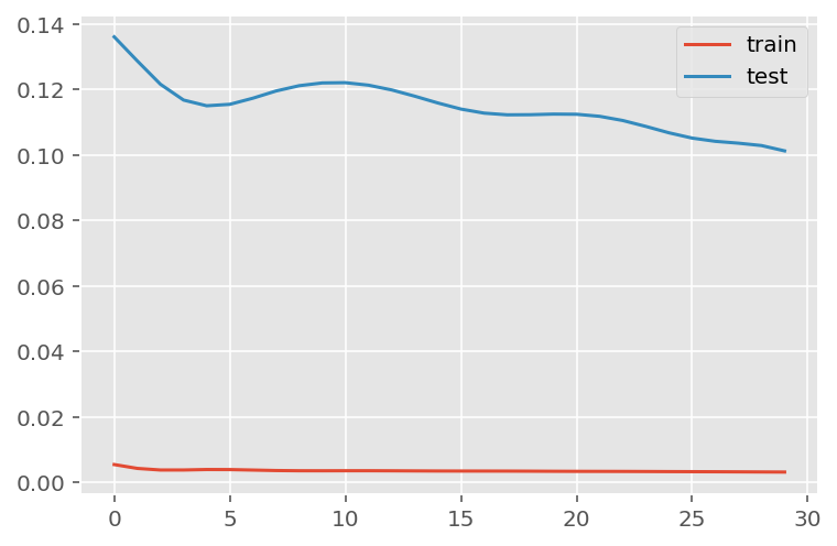 

# Get the predicted values
predictions = model.predict(x_test)
predictions = scaler_pred.inverse_transform(predictions)

1/3 [=========>....................] - ETA: 0s

3/3 [==============================] - ETA: 0s

3/3 [==============================] - 0s 31ms/step

y_test = y_test.reshape(-1,1)
y_test = scaler_pred.inverse_transform(y_test)

# Calculate the mean absolute error (MAE)
mae = mean_absolute_error(y_test, predictions)
print('MAE: ' + str(round(mae, 1)))

# Calculate the root mean squarred error (RMSE)
rmse = np.sqrt(mean_squared_error(y_test,predictions))
print('RMSE: ' + str(round(rmse, 1)))

# Calculate the root mean squarred error (RMSE)
rmse = mean_squared_error(y_test, 
                          predictions,
                          squared = False)
print('RMSE: ' + str(round(rmse, 1)))

MAE: 6872.2
RMSE: 11041.0
RMSE: 11041.0

# Add the difference between the valid and predicted prices
train = data_barcelona[:(len(x_train)+92)]
valid = data_barcelona[(len(x_train)+91):]

valid.insert(1, "Predictions", predictions, True)
valid.insert(1, "Difference", valid["Predictions"] - valid["num_casos"], True)

# Zoom-in to a closer timeframe
# Date from which on the date is displayed
display_start_date = "2021-10-31" 
valid = valid[valid.index > display_start_date]
train = train[train.index > display_start_date]

# Visualize the data
matplotlib.style.use('ggplot')
fig, ax1 = plt.subplots(figsize=(22, 10), sharex=True)

# Data - Train
xt = train.index; 
yt = train[["num_casos"]]
# Data - Test / validation 
xv = valid.index; 
yv = valid[["num_casos", "Predictions"]]

# Plot
plt.title("barcelona: Predictions vs Real infections", fontsize=20)
plt.ylabel("Nº Cases", fontsize=18)

plt.plot(yt, color="blue", linewidth=1.5)
plt.plot(yv["Predictions"], color="red", linewidth=1.5)
plt.plot(yv["num_casos"], color="green", linewidth=1.5)
plt.legend(["Train", "LSTM Predictions", "Test"], 
           loc="upper left", fontsize=18)

# Bar plot with the differences
x = valid.index
y = valid["Difference"]
plt.bar(x, y, width=0.2, color="grey")
plt.grid()
plt.show()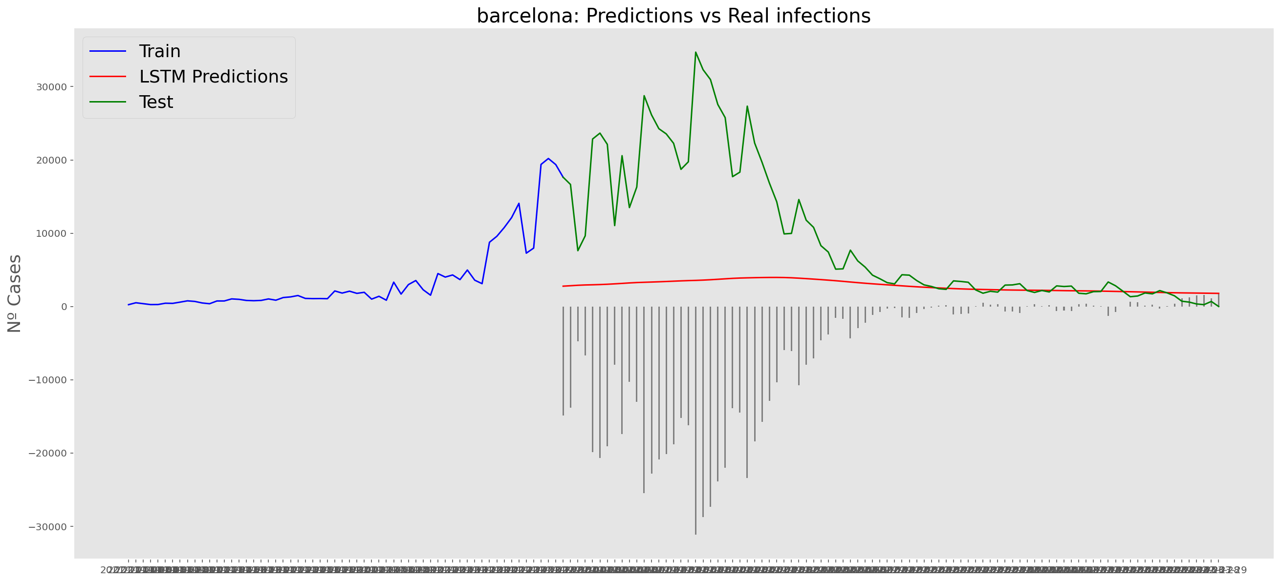

Madrid

data_madrid = data_covid.loc[data_covid['provincia'] == 'Madrid']
data_madrid = data_madrid.set_index('fecha')
data_madrid = data_madrid['2020-06-14':]
data_madrid = data_madrid.filter(['num_casos', 'tmed', 'mob_grocery_pharmacy', 
'mob_parks', 'mob_residential', 'mob_residential', 'mob_transit_stations', 'mob_workplaces'])
data_madrid

	num_casos	tmed	mob_grocery_pharmacy	mob_parks	mob_residential	mob_residential	mob_transit_stations	mob_workplaces
fecha
2020-06-14	81	19.0	-15.0	25.0	7.0	7.0	-43.0	-6.0
2020-06-15	153	20.7	-8.0	34.0	16.0	16.0	-43.0	-47.0
2020-06-16	91	21.0	-8.0	21.0	17.0	17.0	-43.0	-47.0
2020-06-17	93	20.2	-5.0	34.0	17.0	17.0	-42.0	-47.0
2020-06-18	85	21.9	-7.0	30.0	16.0	16.0	-44.0	-47.0
...	...	...	...	...	...	...	...	...
2022-03-25	356	11.0	-1.0	-37.0	5.0	5.0	-19.0	-17.0
2022-03-26	303	10.4	-7.0	-27.0	1.0	1.0	-15.0	-5.0
2022-03-27	77	10.6	-3.0	-17.0	0.0	0.0	-17.0	-2.0
2022-03-28	839	10.2	2.0	-3.0	4.0	4.0	-15.0	-17.0
2022-03-29	6	13.0	1.0	-11.0	4.0	4.0	-16.0	-16.0

654 rows × 8 columns

data_madrid.describe()

	num_casos	tmed	mob_grocery_pharmacy	mob_parks	mob_residential	mob_residential	mob_transit_stations	mob_workplaces
count	654.000000	654.000000	654.000000	654.000000	654.000000	654.000000	654.000000	654.000000
mean	2392.562691	14.909786	-2.608563	-4.874618	6.978593	6.978593	-30.003058	-27.324159
std	3390.272836	8.073496	15.108581	20.826186	5.672763	5.672763	12.389295	18.988563
min	6.000000	-6.200000	-84.000000	-62.000000	-6.000000	-6.000000	-73.000000	-86.000000
25%	662.750000	8.600000	-9.000000	-17.750000	4.000000	4.000000	-39.000000	-40.000000
50%	1413.000000	13.200000	-1.000000	-4.000000	7.000000	7.000000	-31.000000	-26.000000
75%	2475.750000	21.800000	8.000000	11.000000	10.000000	10.000000	-21.000000	-16.000000
max	23811.000000	32.700000	50.000000	77.000000	31.000000	31.000000	1.000000	20.000000

np_data_madrid = data_madrid.values

# Train dataset
scaler = MinMaxScaler(feature_range=(0, 1))
scaled_data_madrid = scaler.fit_transform(np_data_madrid)
print(f'Longitud del conjunto de datos disponible: {len(scaled_data_madrid)}')

Longitud del conjunto de datos disponible: 654

# Since we are going to predict future values based on the 90 past elements, 
# we need to create a list with those historic information for each element
historic_values = 90
scaled_data_madrid_x = []
scaled_data_madrid_y = []

for i in range(historic_values, len(scaled_data_madrid)):
    scaled_data_madrid_x.append(scaled_data_madrid[(i-historic_values):i, :])
    scaled_data_madrid_y.append(scaled_data_madrid[i, 0])

# Convert the x_train and y_train to numpy arrays
scaled_data_madrid_x = np.array(scaled_data_madrid_x)
scaled_data_madrid_y = np.array(scaled_data_madrid_y)

# Once predicted, we are going to need a exclusive scaler for num_cases
scaler_pred = MinMaxScaler(feature_range=(0, 1))
df_cases_madrid = pd.DataFrame(data_madrid['num_casos'])
scaled_data_madrid_pred = scaler_pred.fit_transform(df_cases_madrid)

# Since the first 90th values does not have historic, the dataset has been reduced in 90 values
print(f'Longitud datos de entrenamiento con historico: {len(scaled_data_madrid_y)}')

Longitud datos de entrenamiento con historico: 564

# we split data in train and test
# as in previous analysis, we are going to predict a maximum of 90 days
x_train = scaled_data_madrid_x[0:len(scaled_data_madrid_x)-91]
y_train = scaled_data_madrid_y[0:len(scaled_data_madrid_y)-91]
print(f'Cantidad datos de entrenamiento: x={len(x_train)} - y={len(y_train)}')

x_test = scaled_data_madrid_x[len(scaled_data_madrid_x)-90:len(scaled_data_madrid_x)]
y_test = scaled_data_madrid_y[len(scaled_data_madrid_y)-90:len(scaled_data_madrid_y)]
print(f'Cantidad datos de test: x={len(x_test)} - y={len(y_test)}')

Cantidad datos de entrenamiento: x=473 - y=473
Cantidad datos de test: x=90 - y=90

# Reshape the data to feed de recurrent network
x_train = np.reshape(x_train, (x_train.shape[0], x_train.shape[1], 8))
print("Train data shape:")
print(x_train.shape)
print(y_train.shape)
x_test = np.reshape(x_test, (x_test.shape[0], x_test.shape[1], 8))
print("Test data shape:")
print(x_test.shape)
print(y_test.shape)

Train data shape:
(473, 90, 8)
(473,)
Test data shape:
(90, 90, 8)
(90,)

# Configure / setup the neural network model - LSTM
# Build the model
print('Build model...')
model = Sequential()
# Model with Neurons 
# Inputshape = neurons -> Timestamps
neurons= x_train.shape[1]
model.add(LSTM(90, 
               activation = 'relu',
               return_sequences = True, 
               input_shape = (x_train.shape[1], 8))) 
model.add(LSTM(50, 
               activation = 'relu',
               return_sequences = True)) 
model.add(LSTM(25, 
               activation = 'relu',
               return_sequences = False)) 
model.add(Dense(5, activation = 'relu'))
model.add(Dense(1))

Build model...

model.compile(optimizer='adam', loss='mean_squared_error')
model.summary()

Model: "sequential_2"

_________________________________________________________________

 Layer (type)                Output Shape              Param #   

=================================================================

 lstm_6 (LSTM)               (None, 90, 90)            35640     

 lstm_7 (LSTM)               (None, 90, 50)            28200     

 lstm_8 (LSTM)               (None, 25)                7600      

 dense_4 (Dense)             (None, 5)                 130       

 dense_5 (Dense)             (None, 1)                 6         

=================================================================

Total params: 71,576

Trainable params: 71,576

Non-trainable params: 0

_________________________________________________________________

# Training the model
# fit network
history = model.fit(x_train, 
                    y_train, 
                    batch_size=1000, 
                    epochs=30, 
                    validation_data = (x_test, y_test), 
                    verbose = 0)

plt.plot(history.history['loss'], label='train')
plt.plot(history.history['val_loss'], label='test')
plt.legend()
plt.show()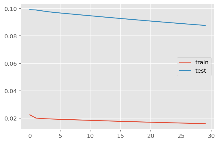 

# Get the predicted values
predictions = model.predict(x_test)
predictions = scaler_pred.inverse_transform(predictions)

1/3 [=========>....................] - ETA: 0s

3/3 [==============================] - ETA: 0s

3/3 [==============================] - 0s 30ms/step

y_test = y_test.reshape(-1,1)
y_test = scaler_pred.inverse_transform(y_test)

# Calculate the mean absolute error (MAE)
mae = mean_absolute_error(y_test, predictions)
print('MAE: ' + str(round(mae, 1)))

# Calculate the root mean squarred error (RMSE)
rmse = np.sqrt(mean_squared_error(y_test,predictions))
print('RMSE: ' + str(round(rmse, 1)))

# Calculate the root mean squarred error (RMSE)
rmse = mean_squared_error(y_test, 
                          predictions,
                          squared = False)
print('RMSE: ' + str(round(rmse, 1)))

MAE: 4531.8
RMSE: 7047.1
RMSE: 7047.1

# Add the difference between the valid and predicted prices
train = data_madrid[:(len(x_train)+92)]
valid = data_madrid[(len(x_train)+91):]

valid.insert(1, "Predictions", predictions, True)
valid.insert(1, "Difference", valid["Predictions"] - valid["num_casos"], True)

# Zoom-in to a closer timeframe
# Date from which on the date is displayed
display_start_date = "2021-10-31" 
valid = valid[valid.index > display_start_date]
train = train[train.index > display_start_date]

# Visualize the data
matplotlib.style.use('ggplot')
fig, ax1 = plt.subplots(figsize=(22, 10), sharex=True)

# Data - Train
xt = train.index; 
yt = train[["num_casos"]]
# Data - Test / validation 
xv = valid.index; 
yv = valid[["num_casos", "Predictions"]]

# Plot
plt.title("madrid: Predictions vs Real infections", fontsize=20)
plt.ylabel("Nº Cases", fontsize=18)

plt.plot(yt, color="blue", linewidth=1.5)
plt.plot(yv["Predictions"], color="red", linewidth=1.5)
plt.plot(yv["num_casos"], color="green", linewidth=1.5)
plt.legend(["Train", "LSTM Predictions", "Test"], 
           loc="upper left", fontsize=18)

# Bar plot with the differences
x = valid.index
y = valid["Difference"]
plt.bar(x, y, width=0.2, color="grey")
plt.grid()
plt.show()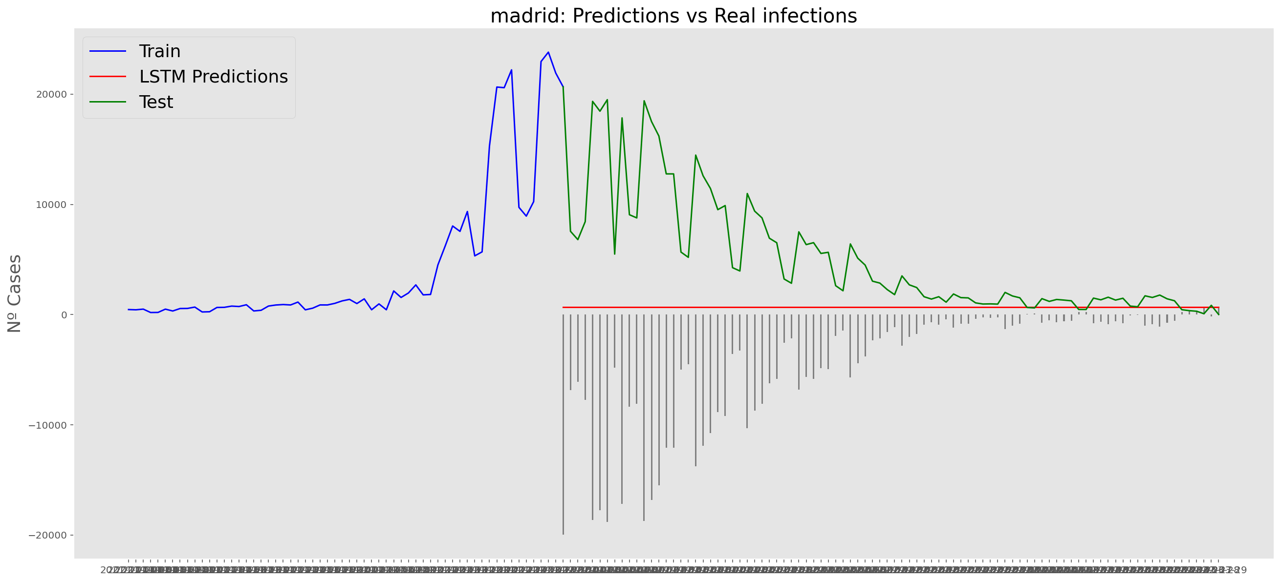

Málaga

data_malaga = data_covid.loc[data_covid['provincia'] == 'Málaga']
data_malaga = data_malaga.set_index('fecha')
data_malaga = data_malaga['2020-06-14':]
data_malaga = data_malaga.filter(['num_casos', 'tmed', 'mob_grocery_pharmacy', 
'mob_parks', 'mob_residential', 'mob_residential', 'mob_transit_stations', 'mob_workplaces'])
data_malaga

	num_casos	tmed	mob_grocery_pharmacy	mob_parks	mob_residential	mob_residential	mob_transit_stations	mob_workplaces
fecha
2020-06-14	2	26.6	-20.0	-15.0	2.0	2.0	-53.0	-7.0
2020-06-15	1	27.2	-16.0	-9.0	9.0	9.0	-44.0	-33.0
2020-06-16	1	27.8	-13.0	-4.0	9.0	9.0	-40.0	-33.0
2020-06-17	2	26.9	-13.0	1.0	9.0	9.0	-41.0	-33.0
2020-06-18	2	21.6	-12.0	3.0	9.0	9.0	-42.0	-33.0
...	...	...	...	...	...	...	...	...
2022-03-25	565	13.8	-3.0	-32.0	8.0	8.0	-18.0	-12.0
2022-03-26	79	14.5	-1.0	-1.0	3.0	3.0	-13.0	-4.0
2022-03-27	65	15.4	5.0	-18.0	2.0	2.0	0.0	0.0
2022-03-28	39	16.3	6.0	-4.0	3.0	3.0	-4.0	-7.0
2022-03-29	0	16.8	4.0	-3.0	4.0	4.0	1.0	-8.0

654 rows × 8 columns

data_malaga.describe()

	num_casos	tmed	mob_grocery_pharmacy	mob_parks	mob_residential	mob_residential	mob_transit_stations	mob_workplaces
count	654.000000	654.000000	654.000000	654.000000	654.000000	654.000000	654.000000	654.00000
mean	410.206422	19.511162	8.776758	13.570336	4.529052	4.529052	-18.853211	-18.04893
std	489.452348	5.721942	26.696909	39.148014	4.064365	4.064365	18.183256	14.55877
min	0.000000	6.200000	-80.000000	-63.000000	-4.000000	-4.000000	-70.000000	-79.00000
25%	122.250000	14.725000	-4.000000	-13.000000	2.000000	2.000000	-32.000000	-26.00000
50%	215.500000	18.400000	6.000000	5.000000	4.000000	4.000000	-21.000000	-17.00000
75%	475.250000	24.500000	15.000000	30.000000	6.750000	6.750000	-4.000000	-11.00000
max	3080.000000	34.500000	156.000000	152.000000	22.000000	22.000000	20.000000	29.00000

np_data_malaga = data_malaga.values

# Train dataset
scaler = MinMaxScaler(feature_range=(0, 1))
scaled_data_malaga = scaler.fit_transform(np_data_malaga)
print(f'Longitud del conjunto de datos disponible: {len(scaled_data_malaga)}')

Longitud del conjunto de datos disponible: 654

# Since we are going to predict future values based on the 90 past elements, 
# we need to create a list with those historic information for each element
historic_values = 90
scaled_data_malaga_x = []
scaled_data_malaga_y = []

for i in range(historic_values, len(scaled_data_malaga)):
    scaled_data_malaga_x.append(scaled_data_malaga[(i-historic_values):i, :])
    scaled_data_malaga_y.append(scaled_data_malaga[i, 0])

# Convert the x_train and y_train to numpy arrays
scaled_data_malaga_x = np.array(scaled_data_malaga_x)
scaled_data_malaga_y = np.array(scaled_data_malaga_y)

# Once predicted, we are going to need a exclusive scaler for num_cases
scaler_pred = MinMaxScaler(feature_range=(0, 1))
df_cases_malaga = pd.DataFrame(data_malaga['num_casos'])
scaled_data_malaga_pred = scaler_pred.fit_transform(df_cases_malaga)

# Since the first 90th values does not have historic, the dataset has been reduced in 90 values
print(f'Longitud datos de entrenamiento con historico: {len(scaled_data_malaga_y)}')

Longitud datos de entrenamiento con historico: 564

# we split data in train and test
# as in previous analysis, we are going to predict a maximum of 90 days
x_train = scaled_data_malaga_x[0:len(scaled_data_malaga_x)-91]
y_train = scaled_data_malaga_y[0:len(scaled_data_malaga_y)-91]
print(f'Cantidad datos de entrenamiento: x={len(x_train)} - y={len(y_train)}')

x_test = scaled_data_malaga_x[len(scaled_data_malaga_x)-90:len(scaled_data_malaga_x)]
y_test = scaled_data_malaga_y[len(scaled_data_malaga_y)-90:len(scaled_data_malaga_y)]
print(f'Cantidad datos de test: x={len(x_test)} - y={len(y_test)}')

Cantidad datos de entrenamiento: x=473 - y=473
Cantidad datos de test: x=90 - y=90

# Reshape the data to feed de recurrent network
x_train = np.reshape(x_train, (x_train.shape[0], x_train.shape[1], 8))
print("Train data shape:")
print(x_train.shape)
print(y_train.shape)
x_test = np.reshape(x_test, (x_test.shape[0], x_test.shape[1], 8))
print("Test data shape:")
print(x_test.shape)
print(y_test.shape)

Train data shape:
(473, 90, 8)
(473,)
Test data shape:
(90, 90, 8)
(90,)

# Configure / setup the neural network model - LSTM
# Build the model
print('Build model...')
model = Sequential()
# Model with Neurons 
# Inputshape = neurons -> Timestamps
neurons= x_train.shape[1]
model.add(LSTM(90, 
               activation = 'relu',
               return_sequences = True, 
               input_shape = (x_train.shape[1], 8))) 
model.add(LSTM(50, 
               activation = 'relu',
               return_sequences = True)) 
model.add(LSTM(25, 
               activation = 'relu',
               return_sequences = False)) 
model.add(Dense(5, activation = 'relu'))
model.add(Dense(1))

Build model...

model.compile(optimizer='adam', loss='mean_squared_error')
model.summary()

Model: "sequential_3"

_________________________________________________________________

 Layer (type)                Output Shape              Param #   

=================================================================

 lstm_9 (LSTM)               (None, 90, 90)            35640     

 lstm_10 (LSTM)              (None, 90, 50)            28200     

 lstm_11 (LSTM)              (None, 25)                7600      

 dense_6 (Dense)             (None, 5)                 130       

 dense_7 (Dense)             (None, 1)                 6         

=================================================================

Total params: 71,576

Trainable params: 71,576

Non-trainable params: 0

_________________________________________________________________

# Training the model
# fit network
history = model.fit(x_train, 
                    y_train, 
                    batch_size=1000, 
                    epochs=30, 
                    validation_data = (x_test, y_test), 
                    verbose = 0)

plt.plot(history.history['loss'], label='train')
plt.plot(history.history['val_loss'], label='test')
plt.legend()
plt.show()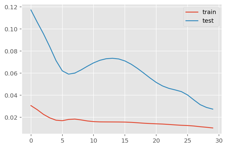 

# Get the predicted values
predictions = model.predict(x_test)
predictions = scaler_pred.inverse_transform(predictions)

1/3 [=========>....................] - ETA: 0s

3/3 [==============================] - ETA: 0s

3/3 [==============================] - 0s 31ms/step

y_test = y_test.reshape(-1,1)
y_test = scaler_pred.inverse_transform(y_test)

# Calculate the mean absolute error (MAE)
mae = mean_absolute_error(y_test, predictions)
print('MAE: ' + str(round(mae, 1)))

# Calculate the root mean squarred error (RMSE)
rmse = np.sqrt(mean_squared_error(y_test,predictions))
print('RMSE: ' + str(round(rmse, 1)))

# Calculate the root mean squarred error (RMSE)
rmse = mean_squared_error(y_test, 
                          predictions,
                          squared = False)
print('RMSE: ' + str(round(rmse, 1)))

MAE: 322.4
RMSE: 508.6
RMSE: 508.6

# Add the difference between the valid and predicted prices
train = data_malaga[:(len(x_train)+92)]
valid = data_malaga[(len(x_train)+91):]

valid.insert(1, "Predictions", predictions, True)
valid.insert(1, "Difference", valid["Predictions"] - valid["num_casos"], True)

# Zoom-in to a closer timeframe
# Date from which on the date is displayed
display_start_date = "2021-10-31" 
valid = valid[valid.index > display_start_date]
train = train[train.index > display_start_date]

# Visualize the data
matplotlib.style.use('ggplot')
fig, ax1 = plt.subplots(figsize=(22, 10), sharex=True)

# Data - Train
xt = train.index; 
yt = train[["num_casos"]]
# Data - Test / validation 
xv = valid.index; 
yv = valid[["num_casos", "Predictions"]]

# Plot
plt.title("malaga: Predictions vs Real infections", fontsize=20)
plt.ylabel("Nº Cases", fontsize=18)

plt.plot(yt, color="blue", linewidth=1.5)
plt.plot(yv["Predictions"], color="red", linewidth=1.5)
plt.plot(yv["num_casos"], color="green", linewidth=1.5)
plt.legend(["Train", "LSTM Predictions", "Test"], 
           loc="upper left", fontsize=18)

# Bar plot with the differences
x = valid.index
y = valid["Difference"]
plt.bar(x, y, width=0.2, color="grey")
plt.grid()
plt.show()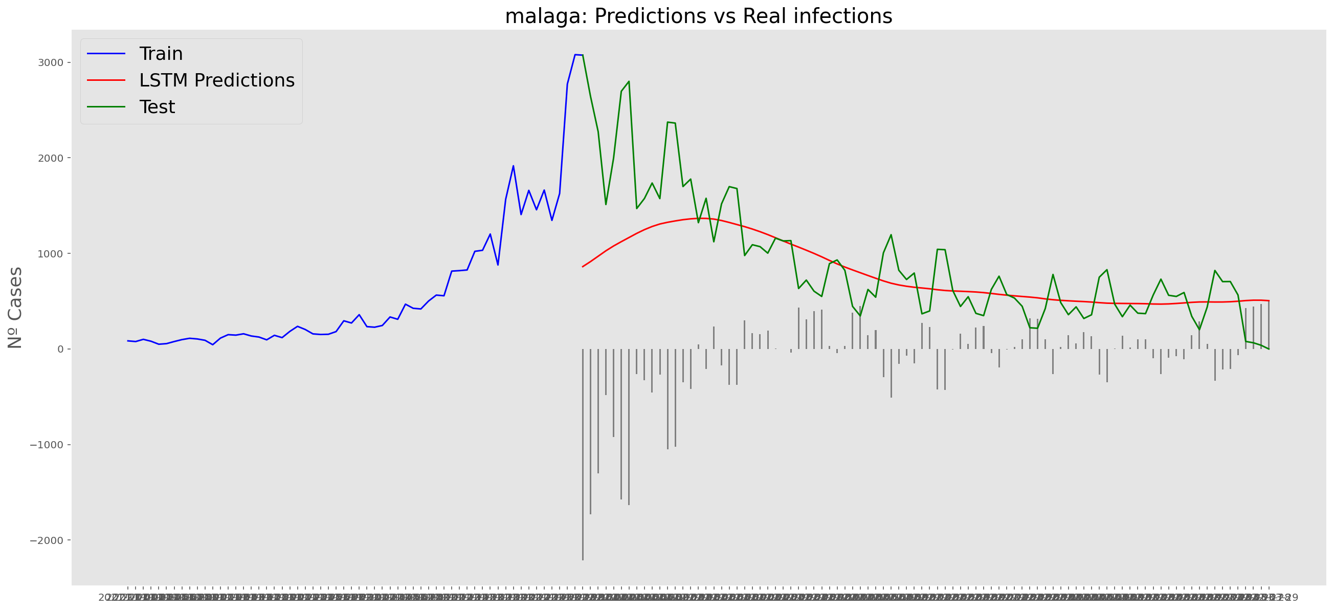

Sevilla

data_sevilla = data_covid.loc[data_covid['provincia'] == 'Sevilla']
data_sevilla = data_sevilla.set_index('fecha')
data_sevilla = data_sevilla['2020-06-14':]
data_sevilla = data_sevilla.filter(['num_casos', 'tmed', 'mob_grocery_pharmacy', 
'mob_parks', 'mob_residential', 'mob_residential', 'mob_transit_stations', 'mob_workplaces'])
data_sevilla

	num_casos	tmed	mob_grocery_pharmacy	mob_parks	mob_residential	mob_residential	mob_transit_stations	mob_workplaces
fecha
2020-06-14	0	22.200000	-24.0	-36.0	0.0	0.0	-51.0	0.0
2020-06-15	2	23.088889	-14.0	-13.0	9.0	9.0	-41.0	-33.0
2020-06-16	1	23.977778	-10.0	-4.0	9.0	9.0	-37.0	-32.0
2020-06-17	0	24.866667	-10.0	-7.0	9.0	9.0	-37.0	-32.0
2020-06-18	0	25.755556	-12.0	-13.0	9.0	9.0	-41.0	-33.0
...	...	...	...	...	...	...	...	...
2022-03-25	365	14.100000	2.0	-20.0	4.0	4.0	-14.0	-7.0
2022-03-26	67	15.200000	-9.0	2.0	0.0	0.0	-12.0	-5.0
2022-03-27	24	15.900000	2.0	-13.0	-1.0	-1.0	-10.0	-7.0
2022-03-28	12	17.100000	2.0	-5.0	2.0	2.0	-10.0	-6.0
2022-03-29	0	16.000000	3.0	-7.0	2.0	2.0	-13.0	-5.0

654 rows × 8 columns

data_sevilla.describe()

	num_casos	tmed	mob_grocery_pharmacy	mob_parks	mob_residential	mob_residential	mob_transit_stations	mob_workplaces
count	654.000000	654.000000	654.000000	654.000000	654.000000	654.000000	654.000000	654.000000
mean	432.978593	19.663609	-0.709480	-14.958716	3.915902	3.915902	-25.707951	-20.347095
std	500.618517	6.949955	18.851349	17.982375	4.397963	4.397963	14.307026	14.434846
min	0.000000	5.500000	-79.000000	-70.000000	-7.000000	-7.000000	-71.000000	-79.000000
25%	127.250000	13.800000	-8.000000	-27.000000	1.000000	1.000000	-36.000000	-29.000000
50%	282.000000	18.600000	0.000000	-13.000000	4.000000	4.000000	-26.000000	-17.000000
75%	528.250000	25.600000	7.000000	-4.000000	6.000000	6.000000	-15.000000	-10.000000
max	3692.000000	34.400000	117.000000	61.000000	22.000000	22.000000	16.000000	9.000000

np_data_sevilla = data_sevilla.values

# Train dataset
scaler = MinMaxScaler(feature_range=(0, 1))
scaled_data_sevilla = scaler.fit_transform(np_data_sevilla)
print(f'Longitud del conjunto de datos disponible: {len(scaled_data_sevilla)}')

Longitud del conjunto de datos disponible: 654

# Since we are going to predict future values based on the 90 past elements, 
# we need to create a list with those historic information for each element
historic_values = 90
scaled_data_sevilla_x = []
scaled_data_sevilla_y = []

for i in range(historic_values, len(scaled_data_sevilla)):
    scaled_data_sevilla_x.append(scaled_data_sevilla[(i-historic_values):i, :])
    scaled_data_sevilla_y.append(scaled_data_sevilla[i, 0])

# Convert the x_train and y_train to numpy arrays
scaled_data_sevilla_x = np.array(scaled_data_sevilla_x)
scaled_data_sevilla_y = np.array(scaled_data_sevilla_y)

# Once predicted, we are going to need a exclusive scaler for num_cases
scaler_pred = MinMaxScaler(feature_range=(0, 1))
df_cases_sevilla = pd.DataFrame(data_sevilla['num_casos'])
scaled_data_sevilla_pred = scaler_pred.fit_transform(df_cases_sevilla)

# Since the first 90th values does not have historic, the dataset has been reduced in 90 values
print(f'Longitud datos de entrenamiento con historico: {len(scaled_data_sevilla_y)}')

Longitud datos de entrenamiento con historico: 564

# we split data in train and test
# as in previous analysis, we are going to predict a maximum of 90 days
x_train = scaled_data_sevilla_x[0:len(scaled_data_sevilla_x)-91]
y_train = scaled_data_sevilla_y[0:len(scaled_data_sevilla_y)-91]
print(f'Cantidad datos de entrenamiento: x={len(x_train)} - y={len(y_train)}')

x_test = scaled_data_sevilla_x[len(scaled_data_sevilla_x)-90:len(scaled_data_sevilla_x)]
y_test = scaled_data_sevilla_y[len(scaled_data_sevilla_y)-90:len(scaled_data_sevilla_y)]
print(f'Cantidad datos de test: x={len(x_test)} - y={len(y_test)}')

Cantidad datos de entrenamiento: x=473 - y=473
Cantidad datos de test: x=90 - y=90

# Reshape the data to feed de recurrent network
x_train = np.reshape(x_train, (x_train.shape[0], x_train.shape[1], 8))
print("Train data shape:")
print(x_train.shape)
print(y_train.shape)
x_test = np.reshape(x_test, (x_test.shape[0], x_test.shape[1], 8))
print("Test data shape:")
print(x_test.shape)
print(y_test.shape)

Train data shape:
(473, 90, 8)
(473,)
Test data shape:
(90, 90, 8)
(90,)

# Configure / setup the neural network model - LSTM
# Build the model
print('Build model...')
model = Sequential()
# Model with Neurons 
# Inputshape = neurons -> Timestamps
neurons= x_train.shape[1]
model.add(LSTM(90, 
               activation = 'relu',
               return_sequences = True, 
               input_shape = (x_train.shape[1], 8))) 
model.add(LSTM(50, 
               activation = 'relu',
               return_sequences = True)) 
model.add(LSTM(25, 
               activation = 'relu',
               return_sequences = False)) 
model.add(Dense(5, activation = 'relu'))
model.add(Dense(1))

Build model...

model.compile(optimizer='adam', loss='mean_squared_error')
model.summary()

Model: "sequential_4"

_________________________________________________________________

 Layer (type)                Output Shape              Param #   

=================================================================

 lstm_12 (LSTM)              (None, 90, 90)            35640     

 lstm_13 (LSTM)              (None, 90, 50)            28200     

 lstm_14 (LSTM)              (None, 25)                7600      

 dense_8 (Dense)             (None, 5)                 130       

 dense_9 (Dense)             (None, 1)                 6         

=================================================================

Total params: 71,576

Trainable params: 71,576

Non-trainable params: 0

_________________________________________________________________

# Training the model
# fit network
history = model.fit(x_train, 
                    y_train, 
                    batch_size=1000, 
                    epochs=30, 
                    validation_data = (x_test, y_test), 
                    verbose = 0)

plt.plot(history.history['loss'], label='train')
plt.plot(history.history['val_loss'], label='test')
plt.legend()
plt.show()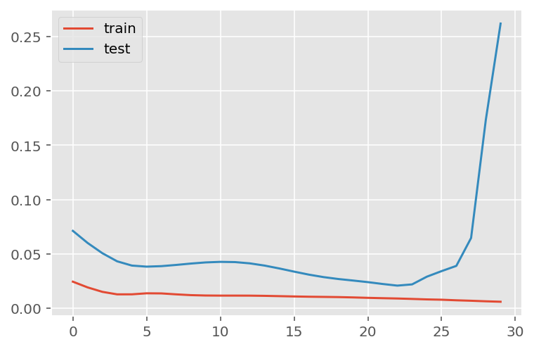 

# Get the predicted values
predictions = model.predict(x_test)
predictions = scaler_pred.inverse_transform(predictions)

WARNING:tensorflow:5 out of the last 13 calls to <function Model.make_predict_function.<locals>.predict_function at 0x7fd54fad4430> triggered tf.function retracing. Tracing is expensive and the excessive number of tracings could be due to (1) creating @tf.function repeatedly in a loop, (2) passing tensors with different shapes, (3) passing Python objects instead of tensors. For (1), please define your @tf.function outside of the loop. For (2), @tf.function has reduce_retracing=True option that can avoid unnecessary retracing. For (3), please refer to https://www.tensorflow.org/guide/function#controlling_retracing and https://www.tensorflow.org/api_docs/python/tf/function for  more details.

1/3 [=========>....................] - ETA: 0s

3/3 [==============================] - ETA: 0s

3/3 [==============================] - 0s 31ms/step

y_test = y_test.reshape(-1,1)
y_test = scaler_pred.inverse_transform(y_test)

# Calculate the mean absolute error (MAE)
mae = mean_absolute_error(y_test, predictions)
print('MAE: ' + str(round(mae, 1)))

# Calculate the root mean squarred error (RMSE)
rmse = np.sqrt(mean_squared_error(y_test,predictions))
print('RMSE: ' + str(round(rmse, 1)))

# Calculate the root mean squarred error (RMSE)
rmse = mean_squared_error(y_test, 
                          predictions,
                          squared = False)
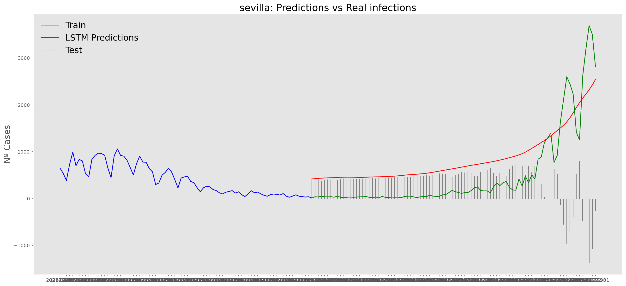
print('RMSE: ' + str(round(rmse, 1)))

MAE: 1622.4
RMSE: 1889.7
RMSE: 1889.7

# Add the difference between the valid and predicted prices
train = data_sevilla[:(len(x_train)+92)]
valid = data_sevilla[(len(x_train)+91):]

valid.insert(1, "Predictions", predictions, True)
valid.insert(1, "Difference", valid["Predictions"] - valid["num_casos"], True)

# Zoom-in to a closer timeframe
# Date from which on the date is displayed
display_start_date = "2021-10-31" 
valid = valid[valid.index > display_start_date]
train = train[train.index > display_start_date]

# Visualize the data
matplotlib.style.use('ggplot')
fig, ax1 = plt.subplots(figsize=(22, 10), sharex=True)

# Data - Train
xt = train.index; 
yt = train[["num_casos"]]
# Data - Test / validation 
xv = valid.index; 
yv = valid[["num_casos", "Predictions"]]

# Plot
plt.title("sevilla: Predictions vs Real infections", fontsize=20)
plt.ylabel("Nº Cases", fontsize=18)

plt.plot(yt, color="blue", linewidth=1.5)
plt.plot(yv["Predictions"], color="red", linewidth=1.5)
plt.plot(yv["num_casos"], color="green", linewidth=1.5)
plt.legend(["Train", "LSTM Predictions", "Test"], 
           loc="upper left", fontsize=18)

# Bar plot with the differences
x = valid.index
y = valid["Difference"]
plt.bar(x, y, width=0.2, color="grey")
plt.grid()
plt.show()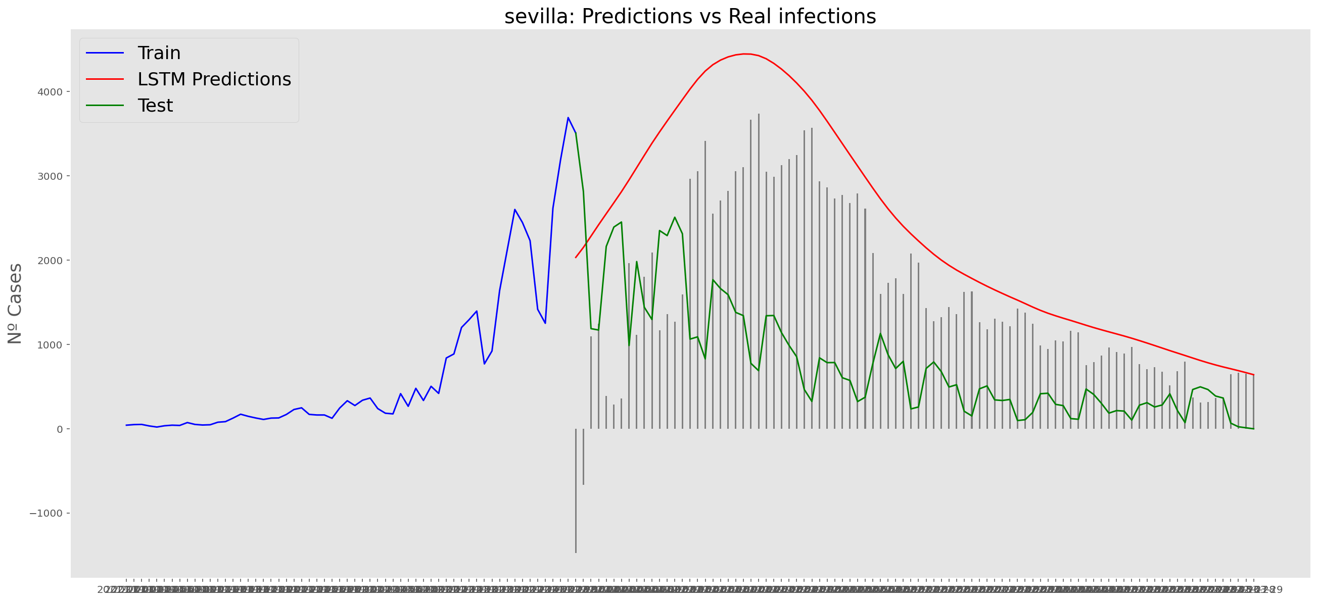

Just before the sixth wave

Asturias

data_asturias = data_covid.loc[data_covid['provincia'] == 'Asturias']
data_asturias = data_asturias.set_index('fecha')
data_asturias = data_asturias['2020-06-14':'2021-12-31']
data_asturias = data_asturias.filter(['num_casos', 'tmed', 'mob_grocery_pharmacy', 
'mob_parks', 'mob_residential', 'mob_residential', 'mob_transit_stations', 'mob_workplaces'])
data_asturias

	num_casos	tmed	mob_grocery_pharmacy	mob_parks	mob_residential	mob_residential	mob_transit_stations	mob_workplaces
fecha
2020-06-14	0	16.8	-8.0	6.0	4.0	4.0	-43.0	-2.0
2020-06-15	0	16.0	-6.0	39.0	7.0	7.0	-38.0	-27.0
2020-06-16	1	15.6	-6.0	7.0	9.0	9.0	-43.0	-29.0
2020-06-17	0	15.6	-7.0	20.0	8.0	8.0	-42.0	-28.0
2020-06-18	0	15.1	-4.0	68.0	7.0	7.0	-39.0	-28.0
...	...	...	...	...	...	...	...	...
2021-12-27	2363	16.6	21.0	57.0	5.0	5.0	-9.0	-35.0
2021-12-28	2150	19.2	18.0	90.0	4.0	4.0	-6.0	-36.0
2021-12-29	2159	15.6	24.0	108.0	4.0	4.0	0.0	-34.0
2021-12-30	2020	13.2	39.0	88.0	4.0	4.0	-10.0	-36.0
2021-12-31	1949	14.6	21.0	46.0	10.0	10.0	-21.0	-54.0

566 rows × 8 columns

data_asturias.describe()

	num_casos	tmed	mob_grocery_pharmacy	mob_parks	mob_residential	mob_residential	mob_transit_stations	mob_workplaces
count	566.000000	566.000000	566.000000	566.000000	566.000000	566.000000	566.000000	566.000000
mean	180.913428	14.495671	4.159011	62.592756	3.798587	3.798587	-12.772085	-21.289753
std	276.250633	4.098429	15.207805	71.365461	5.051424	5.051424	15.668332	13.018468
min	0.000000	3.300000	-87.000000	-63.000000	-8.000000	-8.000000	-67.000000	-80.000000
25%	36.000000	11.525000	-0.375000	14.000000	0.000000	0.000000	-23.000000	-27.000000
50%	94.500000	15.000000	5.000000	43.000000	3.000000	3.000000	-13.000000	-20.000000
75%	225.750000	18.000000	11.000000	91.000000	7.000000	7.000000	-2.000000	-15.000000
max	2363.000000	25.100000	42.000000	333.000000	26.000000	26.000000	26.000000	12.000000

np_data_asturias = data_asturias.values

# Train dataset
scaler = MinMaxScaler(feature_range=(0, 1))
scaled_data_asturias = scaler.fit_transform(np_data_asturias)
print(f'Longitud del conjunto de datos disponible: {len(scaled_data_asturias)}')

Longitud del conjunto de datos disponible: 566

# Since we are going to predict future values based on the 90 past elements, 
# we need to create a list with those historic information for each element
historic_values = 90
scaled_data_asturias_x = []
scaled_data_asturias_y = []

for i in range(historic_values, len(scaled_data_asturias)):
    scaled_data_asturias_x.append(scaled_data_asturias[(i-historic_values):i, :])
    scaled_data_asturias_y.append(scaled_data_asturias[i, 0])

# Convert the x_train and y_train to numpy arrays
scaled_data_asturias_x = np.array(scaled_data_asturias_x)
scaled_data_asturias_y = np.array(scaled_data_asturias_y)

# Once predicted, we are going to need a exclusive scaler for num_cases
scaler_pred = MinMaxScaler(feature_range=(0, 1))
df_cases_asturias = pd.DataFrame(data_asturias['num_casos'])
scaled_data_asturias_pred = scaler_pred.fit_transform(df_cases_asturias)

# Since the first 90th values does not have historic, the dataset has been reduced in 90 values
print(f'Longitud datos de entrenamiento con historico: {len(scaled_data_asturias_y)}')

Longitud datos de entrenamiento con historico: 476

# we split data in train and test
# as in previous analysis, we are going to predict a maximum of 90 days
x_train = scaled_data_asturias_x[0:len(scaled_data_asturias_x)-91]
y_train = scaled_data_asturias_y[0:len(scaled_data_asturias_y)-91]
print(f'Cantidad datos de entrenamiento: x={len(x_train)} - y={len(y_train)}')

x_test = scaled_data_asturias_x[len(scaled_data_asturias_x)-90:len(scaled_data_asturias_x)]
y_test = scaled_data_asturias_y[len(scaled_data_asturias_y)-90:len(scaled_data_asturias_y)]
print(f'Cantidad datos de test: x={len(x_test)} - y={len(y_test)}')

Cantidad datos de entrenamiento: x=385 - y=385
Cantidad datos de test: x=90 - y=90

# Reshape the data to feed de recurrent network
x_train = np.reshape(x_train, (x_train.shape[0], x_train.shape[1], 8))
print("Train data shape:")
print(x_train.shape)
print(y_train.shape)
x_test = np.reshape(x_test, (x_test.shape[0], x_test.shape[1], 8))
print("Test data shape:")
print(x_test.shape)
print(y_test.shape)

Train data shape:
(385, 90, 8)
(385,)
Test data shape:
(90, 90, 8)
(90,)

# Configure / setup the neural network model - LSTM
# Build the model
print('Build model...')
model = Sequential()
# Model with Neurons 
# Inputshape = neurons -> Timestamps
neurons= x_train.shape[1]
model.add(LSTM(90, 
               activation = 'relu',
               return_sequences = True, 
               input_shape = (x_train.shape[1], 8))) 
model.add(LSTM(50, 
               activation = 'relu',
               return_sequences = True)) 
model.add(LSTM(25, 
               activation = 'relu',
               return_sequences = False)) 
model.add(Dense(5, activation = 'relu'))
model.add(Dense(1))

Build model...

model.compile(optimizer='adam', loss='mean_squared_error')
model.summary()

Model: "sequential_5"

_________________________________________________________________

 Layer (type)                Output Shape              Param #   

=================================================================

 lstm_15 (LSTM)              (None, 90, 90)            35640     

 lstm_16 (LSTM)              (None, 90, 50)            28200     

 lstm_17 (LSTM)              (None, 25)                7600      

 dense_10 (Dense)            (None, 5)                 130       

 dense_11 (Dense)            (None, 1)                 6         

=================================================================

Total params: 71,576

Trainable params: 71,576

Non-trainable params: 0

_________________________________________________________________

# Training the model
# fit network
history = model.fit(x_train, 
                    y_train, 
                    batch_size=1000, 
                    epochs=50, 
                    validation_data = (x_test, y_test), 
                    verbose = 0)

plt.plot(history.history['loss'], label='train')
plt.plot(history.history['val_loss'], label='test')
plt.legend()
plt.show()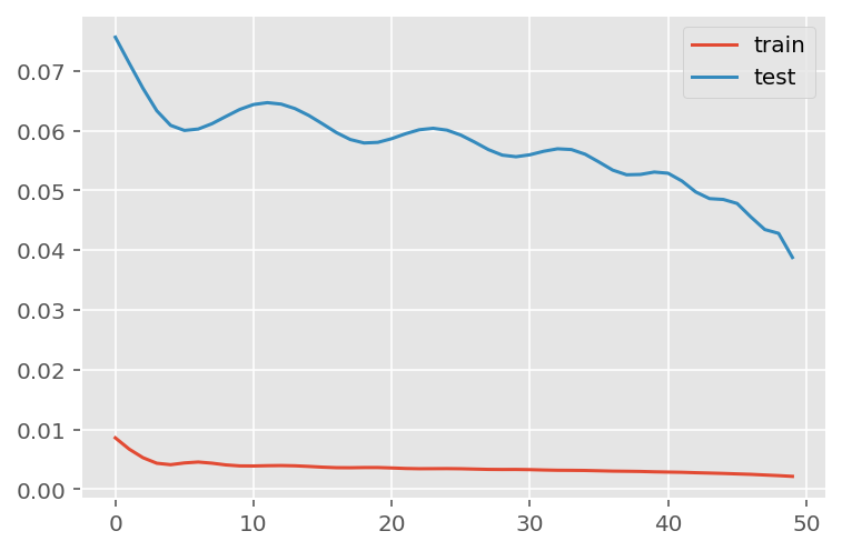 

# Get the predicted values
predictions = model.predict(x_test)
predictions = scaler_pred.inverse_transform(predictions)

WARNING:tensorflow:5 out of the last 13 calls to <function Model.make_predict_function.<locals>.predict_function at 0x7fd53efb6310> triggered tf.function retracing. Tracing is expensive and the excessive number of tracings could be due to (1) creating @tf.function repeatedly in a loop, (2) passing tensors with different shapes, (3) passing Python objects instead of tensors. For (1), please define your @tf.function outside of the loop. For (2), @tf.function has reduce_retracing=True option that can avoid unnecessary retracing. For (3), please refer to https://www.tensorflow.org/guide/function#controlling_retracing and https://www.tensorflow.org/api_docs/python/tf/function for  more details.

1/3 [=========>....................] - ETA: 0s

3/3 [==============================] - ETA: 0s

3/3 [==============================] - 0s 31ms/step

y_test = y_test.reshape(-1,1)
y_test = scaler_pred.inverse_transform(y_test)

# Calculate the mean absolute error (MAE)
mae = mean_absolute_error(y_test, predictions)
print('MAE: ' + str(round(mae, 1)))

# Calculate the root mean squarred error (RMSE)
rmse = np.sqrt(mean_squared_error(y_test,predictions))
print('RMSE: ' + str(round(rmse, 1)))

# Calculate the root mean squarred error (RMSE)
rmse = mean_squared_error(y_test, 
                          predictions,
                          squared = False)
print('RMSE: ' + str(round(rmse, 1)))

MAE: 263.9
RMSE: 465.3
RMSE: 465.3

# Add the difference between the valid and predicted prices
train = data_asturias[:(len(x_train)+92)]
valid = data_asturias[(len(x_train)+91):]

valid.insert(1, "Predictions", predictions, True)
valid.insert(1, "Difference", valid["Predictions"] - valid["num_casos"], True)

# Zoom-in to a closer timeframe
# Date from which on the date is displayed
display_start_date = "2021-07-15" 
valid = valid[valid.index > display_start_date]
train = train[train.index > display_start_date]

# Visualize the data
matplotlib.style.use('ggplot')
fig, ax1 = plt.subplots(figsize=(22, 10), sharex=True)

# Data - Train
xt = train.index; 
yt = train[["num_casos"]]
# Data - Test / validation 
xv = valid.index; 
yv = valid[["num_casos", "Predictions"]]

# Plot
plt.title("Asturias: Predictions vs Real infections", fontsize=20)
plt.ylabel("Nº Cases", fontsize=18)

plt.plot(yt, color="blue", linewidth=1.5)
plt.plot(yv["Predictions"], color="red", linewidth=1.5)
plt.plot(yv["num_casos"], color="green", linewidth=1.5)
plt.legend(["Train", "LSTM Predictions", "Test"], 
           loc="upper left", fontsize=18)

# Bar plot with the differences
x = valid.index
y = valid["Difference"]
plt.bar(x, y, width=0.2, color="grey")
plt.grid()
plt.show()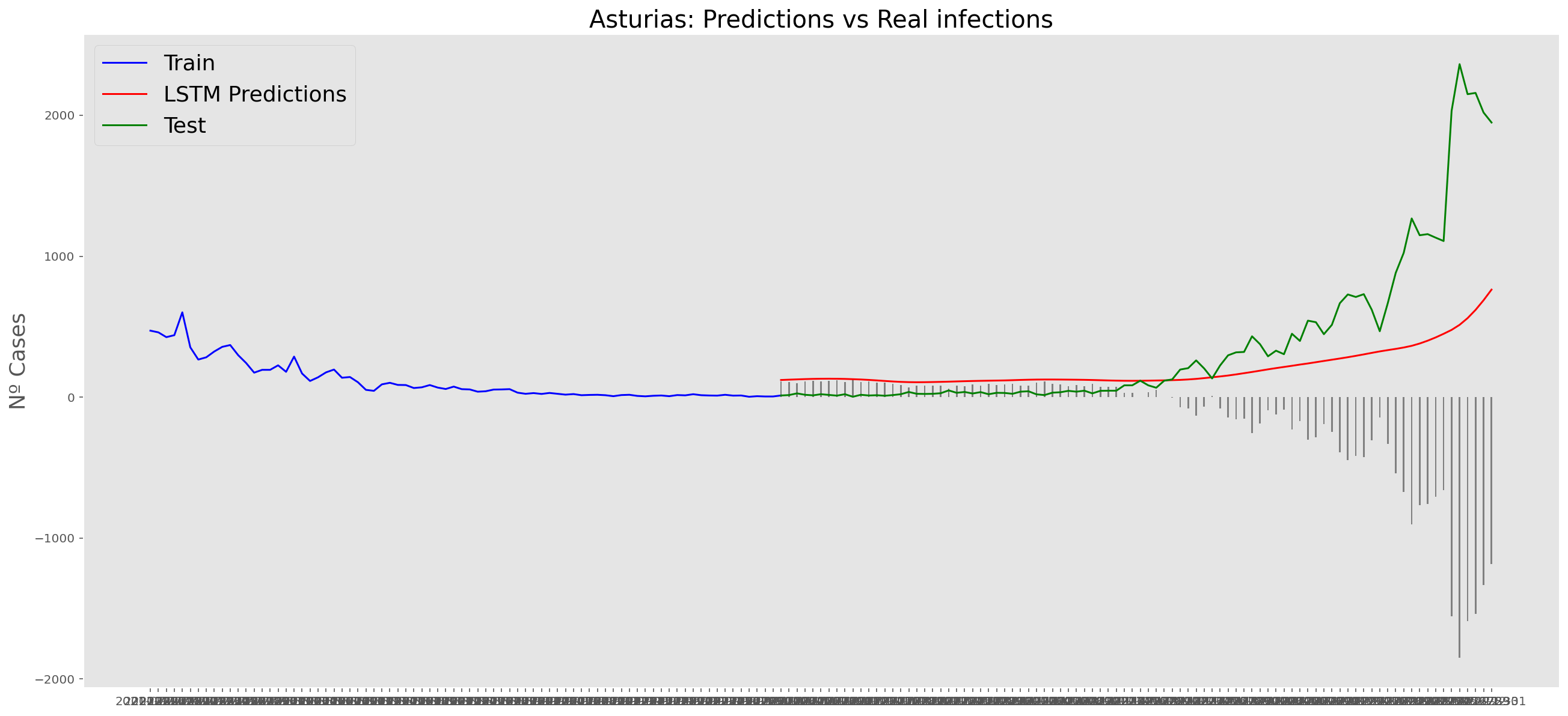

Barcelona

data_barcelona = data_covid.loc[data_covid['provincia'] == 'Barcelona']
data_barcelona = data_barcelona.set_index('fecha')
data_barcelona = data_barcelona['2020-06-14':'2021-12-31']
data_barcelona = data_barcelona.filter(['num_casos', 'tmed', 'mob_grocery_pharmacy', 
'mob_parks', 'mob_residential', 'mob_residential', 'mob_transit_stations', 'mob_workplaces'])
data_barcelona

	num_casos	tmed	mob_grocery_pharmacy	mob_parks	mob_residential	mob_residential	mob_transit_stations	mob_workplaces
fecha
2020-06-14	33	20.6	-20.0	15.0	6.0	6.0	-31.0	-6.0
2020-06-15	62	21.2	-9.0	17.0	14.0	14.0	-34.0	-41.0
2020-06-16	66	20.8	-10.0	-16.0	16.0	16.0	-39.0	-41.0
2020-06-17	70	20.3	-4.0	14.0	15.0	15.0	-33.0	-40.0
2020-06-18	68	18.8	-8.0	-6.0	16.0	16.0	-38.0	-41.0
...	...	...	...	...	...	...	...	...
2021-12-27	19383	16.4	15.0	7.0	12.0	12.0	-25.0	-52.0
2021-12-28	20192	17.7	17.0	7.0	13.0	13.0	-25.0	-52.0
2021-12-29	19361	17.0	23.0	10.0	13.0	13.0	-25.0	-51.0
2021-12-30	17639	15.8	37.0	6.0	12.0	12.0	-24.0	-53.0
2021-12-31	16651	13.6	26.0	-12.0	16.0	16.0	-36.0	-60.0

566 rows × 8 columns

data_barcelona.describe()

	num_casos	tmed	mob_grocery_pharmacy	mob_parks	mob_residential	mob_residential	mob_transit_stations	mob_workplaces
count	566.000000	566.000000	566.000000	566.000000	566.000000	566.000000	566.000000	566.000000
mean	1575.480565	18.205477	-0.574205	-4.651943	7.353357	7.353357	-24.865724	-28.471731
std	2281.290383	6.086976	16.775476	15.728472	5.162377	5.162377	11.574598	16.238872
min	33.000000	4.300000	-83.000000	-76.000000	-6.000000	-6.000000	-72.000000	-87.000000
25%	544.750000	12.800000	-7.000000	-14.750000	4.000000	4.000000	-33.000000	-36.000000
50%	944.500000	17.800000	0.500000	-4.000000	8.000000	8.000000	-25.000000	-26.000000
75%	1609.500000	24.375000	10.000000	7.000000	10.000000	10.000000	-15.000000	-19.250000
max	20192.000000	28.400000	58.000000	33.000000	32.000000	32.000000	-2.000000	6.000000

np_data_barcelona = data_barcelona.values

# Train dataset
scaler = MinMaxScaler(feature_range=(0, 1))
scaled_data_barcelona = scaler.fit_transform(np_data_barcelona)
print(f'Longitud del conjunto de datos disponible: {len(scaled_data_barcelona)}')

Longitud del conjunto de datos disponible: 566

# Since we are going to predict future values based on the 90 past elements, 
# we need to create a list with those historic information for each element
historic_values = 90
scaled_data_barcelona_x = []
scaled_data_barcelona_y = []

for i in range(historic_values, len(scaled_data_barcelona)):
    scaled_data_barcelona_x.append(scaled_data_barcelona[(i-historic_values):i, :])
    scaled_data_barcelona_y.append(scaled_data_barcelona[i, 0])

# Convert the x_train and y_train to numpy arrays
scaled_data_barcelona_x = np.array(scaled_data_barcelona_x)
scaled_data_barcelona_y = np.array(scaled_data_barcelona_y)

# Once predicted, we are going to need a exclusive scaler for num_cases
scaler_pred = MinMaxScaler(feature_range=(0, 1))
df_cases_barcelona = pd.DataFrame(data_barcelona['num_casos'])
scaled_data_barcelona_pred = scaler_pred.fit_transform(df_cases_barcelona)

# Since the first 90th values does not have historic, the dataset has been reduced in 90 values
print(f'Longitud datos de entrenamiento con historico: {len(scaled_data_barcelona_y)}')

Longitud datos de entrenamiento con historico: 476

# we split data in train and test
# as in previous analysis, we are going to predict a maximum of 90 days
x_train = scaled_data_barcelona_x[0:len(scaled_data_barcelona_x)-91]
y_train = scaled_data_barcelona_y[0:len(scaled_data_barcelona_y)-91]
print(f'Cantidad datos de entrenamiento: x={len(x_train)} - y={len(y_train)}')

x_test = scaled_data_barcelona_x[len(scaled_data_barcelona_x)-90:len(scaled_data_barcelona_x)]
y_test = scaled_data_barcelona_y[len(scaled_data_barcelona_y)-90:len(scaled_data_barcelona_y)]
print(f'Cantidad datos de test: x={len(x_test)} - y={len(y_test)}')

Cantidad datos de entrenamiento: x=385 - y=385
Cantidad datos de test: x=90 - y=90

# Reshape the data to feed de recurrent network
x_train = np.reshape(x_train, (x_train.shape[0], x_train.shape[1], 8))
print("Train data shape:")
print(x_train.shape)
print(y_train.shape)
x_test = np.reshape(x_test, (x_test.shape[0], x_test.shape[1], 8))
print("Test data shape:")
print(x_test.shape)
print(y_test.shape)

Train data shape:
(385, 90, 8)
(385,)
Test data shape:
(90, 90, 8)
(90,)

# Configure / setup the neural network model - LSTM
# Build the model
print('Build model...')
model = Sequential()
# Model with Neurons 
# Inputshape = neurons -> Timestamps
neurons= x_train.shape[1]
model.add(LSTM(90, 
               activation = 'relu',
               return_sequences = True, 
               input_shape = (x_train.shape[1], 8))) 
model.add(LSTM(50, 
               activation = 'relu',
               return_sequences = True)) 
model.add(LSTM(25, 
               activation = 'relu',
               return_sequences = False)) 
model.add(Dense(5, activation = 'relu'))
model.add(Dense(1))

Build model...

model.compile(optimizer='adam', loss='mean_squared_error')
model.summary()

Model: "sequential_6"

_________________________________________________________________

 Layer (type)                Output Shape              Param #   

=================================================================

 lstm_18 (LSTM)              (None, 90, 90)            35640     

 lstm_19 (LSTM)              (None, 90, 50)            28200     

 lstm_20 (LSTM)              (None, 25)                7600      

 dense_12 (Dense)            (None, 5)                 130       

 dense_13 (Dense)            (None, 1)                 6         

=================================================================

Total params: 71,576

Trainable params: 71,576

Non-trainable params: 0

_________________________________________________________________

# Training the model
# fit network
history = model.fit(x_train, 
                    y_train, 
                    batch_size=1000, 
                    epochs=50, 
                    validation_data = (x_test, y_test), 
                    verbose = 0)

plt.plot(history.history['loss'], label='train')
plt.plot(history.history['val_loss'], label='test')
plt.legend()
plt.show()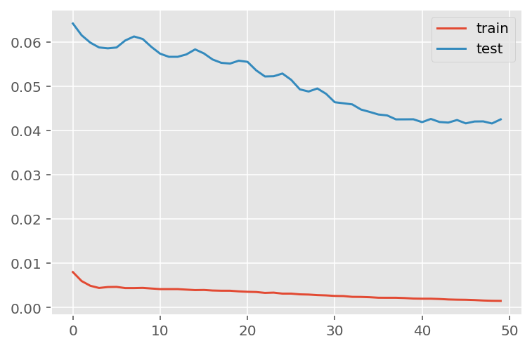 

# Get the predicted values
predictions = model.predict(x_test)
predictions = scaler_pred.inverse_transform(predictions)

1/3 [=========>....................] - ETA: 0s

3/3 [==============================] - ETA: 0s

3/3 [==============================] - 0s 31ms/step

y_test = y_test.reshape(-1,1)
y_test = scaler_pred.inverse_transform(y_test)

# Calculate the mean absolute error (MAE)
mae = mean_absolute_error(y_test, predictions)
print('MAE: ' + str(round(mae, 1)))

# Calculate the root mean squarred error (RMSE)
rmse = np.sqrt(mean_squared_error(y_test,predictions))
print('RMSE: ' + str(round(rmse, 1)))

# Calculate the root mean squarred error (RMSE)
rmse = mean_squared_error(y_test, 
                          predictions,
                          squared = False)
print('RMSE: ' + str(round(rmse, 1)))

MAE: 2657.6
RMSE: 4156.6
RMSE: 4156.6

# Add the difference between the valid and predicted prices
train = data_barcelona[:(len(x_train)+92)]
valid = data_barcelona[(len(x_train)+91):]

valid.insert(1, "Predictions", predictions, True)
valid.insert(1, "Difference", valid["Predictions"] - valid["num_casos"], True)

# Zoom-in to a closer timeframe
# Date from which on the date is displayed
display_start_date = "2021-07-15" 
valid = valid[valid.index > display_start_date]
train = train[train.index > display_start_date]

# Visualize the data
matplotlib.style.use('ggplot')
fig, ax1 = plt.subplots(figsize=(22, 10), sharex=True)

# Data - Train
xt = train.index; 
yt = train[["num_casos"]]
# Data - Test / validation 
xv = valid.index; 
yv = valid[["num_casos", "Predictions"]]

# Plot
plt.title("barcelona: Predictions vs Real infections", fontsize=20)
plt.ylabel("Nº Cases", fontsize=18)

plt.plot(yt, color="blue", linewidth=1.5)
plt.plot(yv["Predictions"], color="red", linewidth=1.5)
plt.plot(yv["num_casos"], color="green", linewidth=1.5)
plt.legend(["Train", "LSTM Predictions", "Test"], 
           loc="upper left", fontsize=18)

# Bar plot with the differences
x = valid.index
y = valid["Difference"]
plt.bar(x, y, width=0.2, color="grey")
plt.grid()
plt.show()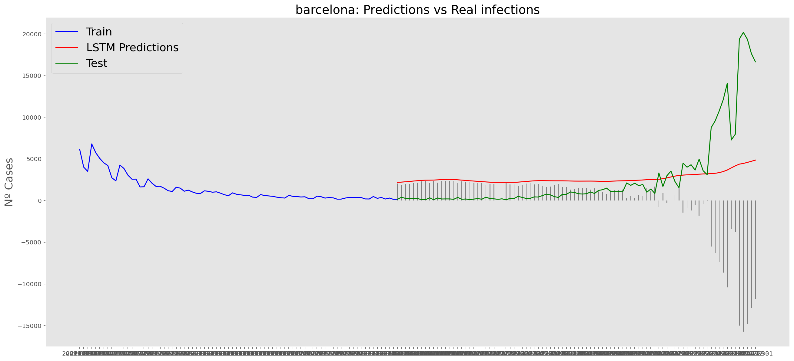

Madrid

data_madrid = data_covid.loc[data_covid['provincia'] == 'Madrid']
data_madrid = data_madrid.set_index('fecha')
data_madrid = data_madrid['2020-06-14':'2021-12-31']
data_madrid = data_madrid.filter(['num_casos', 'tmed', 'mob_grocery_pharmacy', 
'mob_parks', 'mob_residential', 'mob_residential', 'mob_transit_stations', 'mob_workplaces'])
data_madrid

	num_casos	tmed	mob_grocery_pharmacy	mob_parks	mob_residential	mob_residential	mob_transit_stations	mob_workplaces
fecha
2020-06-14	81	19.0	-15.0	25.0	7.0	7.0	-43.0	-6.0
2020-06-15	153	20.7	-8.0	34.0	16.0	16.0	-43.0	-47.0
2020-06-16	91	21.0	-8.0	21.0	17.0	17.0	-43.0	-47.0
2020-06-17	93	20.2	-5.0	34.0	17.0	17.0	-42.0	-47.0
2020-06-18	85	21.9	-7.0	30.0	16.0	16.0	-44.0	-47.0
...	...	...	...	...	...	...	...	...
2021-12-27	22958	12.3	21.0	19.0	12.0	12.0	-28.0	-52.0
2021-12-28	23811	10.4	18.0	23.0	12.0	12.0	-30.0	-52.0
2021-12-29	21914	9.0	27.0	18.0	13.0	13.0	-30.0	-52.0
2021-12-30	20666	8.7	42.0	17.0	12.0	12.0	-30.0	-53.0
2021-12-31	7556	9.2	10.0	-15.0	18.0	18.0	-47.0	-69.0

566 rows × 8 columns

data_madrid.describe()

	num_casos	tmed	mob_grocery_pharmacy	mob_parks	mob_residential	mob_residential	mob_transit_stations	mob_workplaces
count	566.000000	566.000000	566.000000	566.000000	566.000000	566.000000	566.000000	566.000000
mean	1994.136042	16.004064	-3.793286	-4.438163	7.238516	7.238516	-31.560071	-28.715548
std	2795.419848	8.085617	14.945139	21.384112	5.850467	5.850467	12.292703	19.230654
min	28.000000	-6.200000	-84.000000	-62.000000	-6.000000	-6.000000	-73.000000	-86.000000
25%	550.250000	9.525000	-11.000000	-17.750000	4.000000	4.000000	-40.000000	-41.000000
50%	1312.500000	14.700000	-3.000000	-3.000000	7.000000	7.000000	-33.000000	-28.000000
75%	2282.500000	23.200000	6.000000	11.750000	11.000000	11.000000	-24.000000	-17.000000
max	23811.000000	32.700000	50.000000	77.000000	31.000000	31.000000	1.000000	20.000000

np_data_madrid = data_madrid.values

# Train dataset
scaler = MinMaxScaler(feature_range=(0, 1))
scaled_data_madrid = scaler.fit_transform(np_data_madrid)
print(f'Longitud del conjunto de datos disponible: {len(scaled_data_madrid)}')

Longitud del conjunto de datos disponible: 566

# Since we are going to predict future values based on the 90 past elements, 
# we need to create a list with those historic information for each element
historic_values = 90
scaled_data_madrid_x = []
scaled_data_madrid_y = []

for i in range(historic_values, len(scaled_data_madrid)):
    scaled_data_madrid_x.append(scaled_data_madrid[(i-historic_values):i, :])
    scaled_data_madrid_y.append(scaled_data_madrid[i, 0])

# Convert the x_train and y_train to numpy arrays
scaled_data_madrid_x = np.array(scaled_data_madrid_x)
scaled_data_madrid_y = np.array(scaled_data_madrid_y)

# Once predicted, we are going to need a exclusive scaler for num_cases
scaler_pred = MinMaxScaler(feature_range=(0, 1))
df_cases_madrid = pd.DataFrame(data_madrid['num_casos'])
scaled_data_madrid_pred = scaler_pred.fit_transform(df_cases_madrid)

# Since the first 90th values does not have historic, the dataset has been reduced in 90 values
print(f'Longitud datos de entrenamiento con historico: {len(scaled_data_madrid_y)}')

Longitud datos de entrenamiento con historico: 476

# we split data in train and test
# as in previous analysis, we are going to predict a maximum of 90 days
x_train = scaled_data_madrid_x[0:len(scaled_data_madrid_x)-91]
y_train = scaled_data_madrid_y[0:len(scaled_data_madrid_y)-91]
print(f'Cantidad datos de entrenamiento: x={len(x_train)} - y={len(y_train)}')

x_test = scaled_data_madrid_x[len(scaled_data_madrid_x)-90:len(scaled_data_madrid_x)]
y_test = scaled_data_madrid_y[len(scaled_data_madrid_y)-90:len(scaled_data_madrid_y)]
print(f'Cantidad datos de test: x={len(x_test)} - y={len(y_test)}')

Cantidad datos de entrenamiento: x=385 - y=385
Cantidad datos de test: x=90 - y=90

# Reshape the data to feed de recurrent network
x_train = np.reshape(x_train, (x_train.shape[0], x_train.shape[1], 8))
print("Train data shape:")
print(x_train.shape)
print(y_train.shape)
x_test = np.reshape(x_test, (x_test.shape[0], x_test.shape[1], 8))
print("Test data shape:")
print(x_test.shape)
print(y_test.shape)

Train data shape:
(385, 90, 8)
(385,)
Test data shape:
(90, 90, 8)
(90,)

# Configure / setup the neural network model - LSTM
# Build the model
print('Build model...')
model = Sequential()
# Model with Neurons 
# Inputshape = neurons -> Timestamps
neurons= x_train.shape[1]
model.add(LSTM(90, 
               activation = 'relu',
               return_sequences = True, 
               input_shape = (x_train.shape[1], 8))) 
model.add(LSTM(50, 
               activation = 'relu',
               return_sequences = True)) 
model.add(LSTM(25, 
               activation = 'relu',
               return_sequences = False)) 
model.add(Dense(5, activation = 'relu'))
model.add(Dense(1))

Build model...

model.compile(optimizer='adam', loss='mean_squared_error')
model.summary()

Model: "sequential_7"

_________________________________________________________________

 Layer (type)                Output Shape              Param #   

=================================================================

 lstm_21 (LSTM)              (None, 90, 90)            35640     

 lstm_22 (LSTM)              (None, 90, 50)            28200     

 lstm_23 (LSTM)              (None, 25)                7600      

 dense_14 (Dense)            (None, 5)                 130       

 dense_15 (Dense)            (None, 1)                 6         

=================================================================

Total params: 71,576

Trainable params: 71,576

Non-trainable params: 0

_________________________________________________________________

# Training the model
# fit network
history = model.fit(x_train, 
                    y_train, 
                    batch_size=1000, 
                    epochs=50, 
                    validation_data = (x_test, y_test), 
                    verbose = 0)

plt.plot(history.history['loss'], label='train')
plt.plot(history.history['val_loss'], label='test')
plt.legend()
plt.show()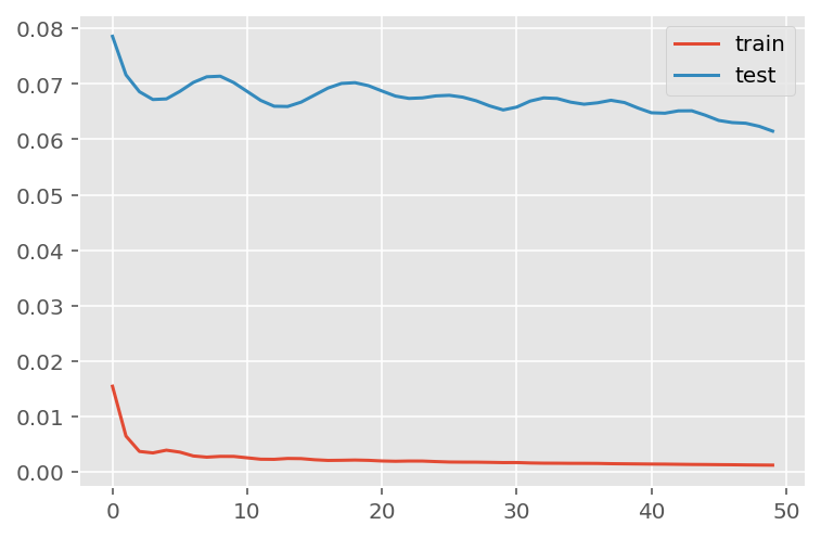 

# Get the predicted values
predictions = model.predict(x_test)
predictions = scaler_pred.inverse_transform(predictions)

1/3 [=========>....................] - ETA: 0s

3/3 [==============================] - ETA: 0s

3/3 [==============================] - 0s 31ms/step

y_test = y_test.reshape(-1,1)
y_test = scaler_pred.inverse_transform(y_test)

# Calculate the mean absolute error (MAE)
mae = mean_absolute_error(y_test, predictions)
print('MAE: ' + str(round(mae, 1)))

# Calculate the root mean squarred error (RMSE)
rmse = np.sqrt(mean_squared_error(y_test,predictions))
print('RMSE: ' + str(round(rmse, 1)))

# Calculate the root mean squarred error (RMSE)
rmse = mean_squared_error(y_test, 
                          predictions,
                          squared = False)
print('RMSE: ' + str(round(rmse, 1)))

MAE: 2755.3
RMSE: 5897.2
RMSE: 5897.2

# Add the difference between the valid and predicted prices
train = data_madrid[:(len(x_train)+92)]
valid = data_madrid[(len(x_train)+91):]

valid.insert(1, "Predictions", predictions, True)
valid.insert(1, "Difference", valid["Predictions"] - valid["num_casos"], True)

# Zoom-in to a closer timeframe
# Date from which on the date is displayed
display_start_date = "2021-07-15" 
valid = valid[valid.index > display_start_date]
train = train[train.index > display_start_date]

# Visualize the data
matplotlib.style.use('ggplot')
fig, ax1 = plt.subplots(figsize=(22, 10), sharex=True)

# Data - Train
xt = train.index; 
yt = train[["num_casos"]]
# Data - Test / validation 
xv = valid.index; 
yv = valid[["num_casos", "Predictions"]]

# Plot
plt.title("madrid: Predictions vs Real infections", fontsize=20)
plt.ylabel("Nº Cases", fontsize=18)

plt.plot(yt, color="blue", linewidth=1.5)
plt.plot(yv["Predictions"], color="red", linewidth=1.5)
plt.plot(yv["num_casos"], color="green", linewidth=1.5)
plt.legend(["Train", "LSTM Predictions", "Test"], 
           loc="upper left", fontsize=18)

# Bar plot with the differences
x = valid.index
y = valid["Difference"]
plt.bar(x, y, width=0.2, color="grey")
plt.grid()
plt.show()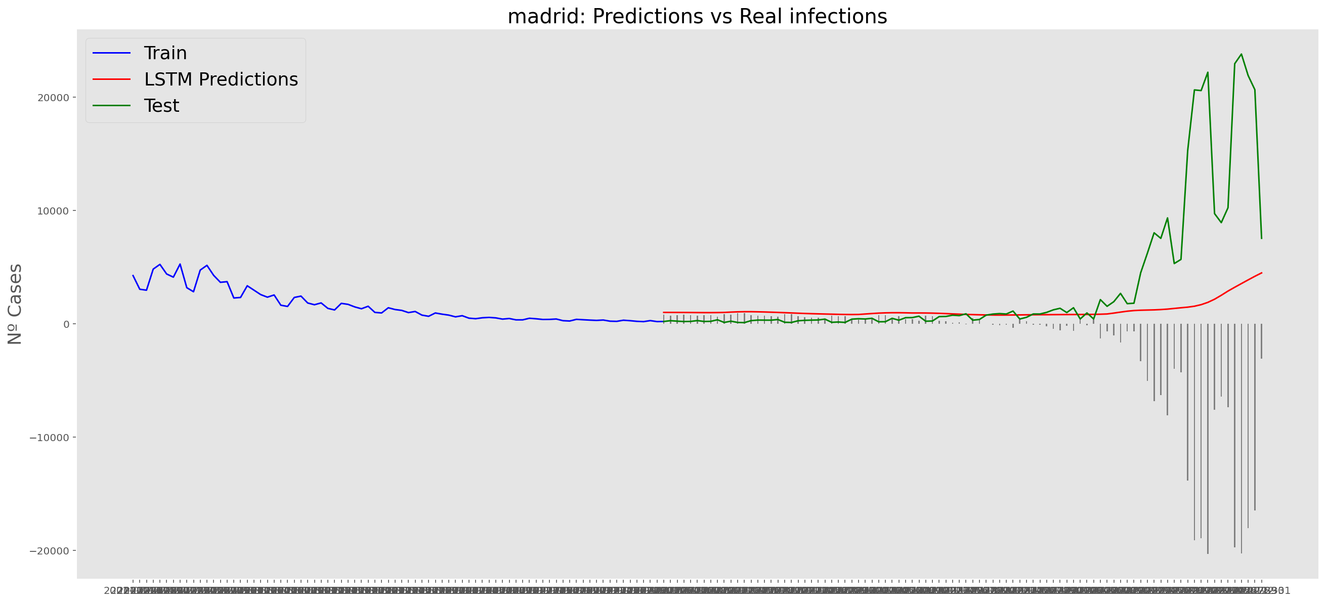

Málaga

data_malaga = data_covid.loc[data_covid['provincia'] == 'Málaga']
data_malaga = data_malaga.set_index('fecha')
data_malaga = data_malaga['2020-06-14':'2021-12-31']
data_malaga = data_malaga.filter(['num_casos', 'tmed', 'mob_grocery_pharmacy', 
'mob_parks', 'mob_residential', 'mob_residential', 'mob_transit_stations', 'mob_workplaces'])
data_malaga

	num_casos	tmed	mob_grocery_pharmacy	mob_parks	mob_residential	mob_residential	mob_transit_stations	mob_workplaces
fecha
2020-06-14	2	26.6	-20.0	-15.0	2.0	2.0	-53.0	-7.0
2020-06-15	1	27.2	-16.0	-9.0	9.0	9.0	-44.0	-33.0
2020-06-16	1	27.8	-13.0	-4.0	9.0	9.0	-40.0	-33.0
2020-06-17	2	26.9	-13.0	1.0	9.0	9.0	-41.0	-33.0
2020-06-18	2	21.6	-12.0	3.0	9.0	9.0	-42.0	-33.0
...	...	...	...	...	...	...	...	...
2021-12-27	1627	17.9	15.0	17.0	7.0	7.0	-12.0	-37.0
2021-12-28	2772	17.8	18.0	30.0	7.0	7.0	-7.0	-37.0
2021-12-29	3080	17.0	25.0	37.0	6.0	6.0	-8.0	-37.0
2021-12-30	3075	14.4	39.0	33.0	5.0	5.0	-8.0	-37.0
2021-12-31	2646	11.1	22.0	-5.0	12.0	12.0	-34.0	-50.0

566 rows × 8 columns

data_malaga.describe()

	num_casos	tmed	mob_grocery_pharmacy	mob_parks	mob_residential	mob_residential	mob_transit_stations	mob_workplaces
count	566.000000	566.000000	566.000000	566.000000	566.000000	566.000000	566.000000	566.000000
mean	339.227915	20.332332	8.427562	15.765018	4.588339	4.588339	-19.860424	-18.724382
std	427.261346	5.690349	27.032414	41.263233	4.227823	4.227823	19.025924	14.733563
min	1.000000	6.200000	-80.000000	-63.000000	-4.000000	-4.000000	-70.000000	-79.000000
25%	110.000000	15.600000	-5.000000	-14.000000	2.000000	2.000000	-34.000000	-27.000000
50%	193.500000	20.000000	4.000000	7.000000	4.000000	4.000000	-23.000000	-18.000000
75%	344.750000	25.075000	16.000000	36.000000	7.000000	7.000000	-4.000000	-12.000000
max	3080.000000	34.500000	156.000000	152.000000	22.000000	22.000000	20.000000	29.000000

np_data_malaga = data_malaga.values

# Train dataset
scaler = MinMaxScaler(feature_range=(0, 1))
scaled_data_malaga = scaler.fit_transform(np_data_malaga)
print(f'Longitud del conjunto de datos disponible: {len(scaled_data_malaga)}')

Longitud del conjunto de datos disponible: 566

# Since we are going to predict future values based on the 90 past elements, 
# we need to create a list with those historic information for each element
historic_values = 90
scaled_data_malaga_x = []
scaled_data_malaga_y = []

for i in range(historic_values, len(scaled_data_malaga)):
    scaled_data_malaga_x.append(scaled_data_malaga[(i-historic_values):i, :])
    scaled_data_malaga_y.append(scaled_data_malaga[i, 0])

# Convert the x_train and y_train to numpy arrays
scaled_data_malaga_x = np.array(scaled_data_malaga_x)
scaled_data_malaga_y = np.array(scaled_data_malaga_y)

# Once predicted, we are going to need a exclusive scaler for num_cases
scaler_pred = MinMaxScaler(feature_range=(0, 1))
df_cases_malaga = pd.DataFrame(data_malaga['num_casos'])
scaled_data_malaga_pred = scaler_pred.fit_transform(df_cases_malaga)

# Since the first 90th values does not have historic, the dataset has been reduced in 90 values
print(f'Longitud datos de entrenamiento con historico: {len(scaled_data_malaga_y)}')

Longitud datos de entrenamiento con historico: 476

# we split data in train and test
# as in previous analysis, we are going to predict a maximum of 90 days
x_train = scaled_data_malaga_x[0:len(scaled_data_malaga_x)-91]
y_train = scaled_data_malaga_y[0:len(scaled_data_malaga_y)-91]
print(f'Cantidad datos de entrenamiento: x={len(x_train)} - y={len(y_train)}')

x_test = scaled_data_malaga_x[len(scaled_data_malaga_x)-90:len(scaled_data_malaga_x)]
y_test = scaled_data_malaga_y[len(scaled_data_malaga_y)-90:len(scaled_data_malaga_y)]
print(f'Cantidad datos de test: x={len(x_test)} - y={len(y_test)}')

Cantidad datos de entrenamiento: x=385 - y=385
Cantidad datos de test: x=90 - y=90

# Reshape the data to feed de recurrent network
x_train = np.reshape(x_train, (x_train.shape[0], x_train.shape[1], 8))
print("Train data shape:")
print(x_train.shape)
print(y_train.shape)
x_test = np.reshape(x_test, (x_test.shape[0], x_test.shape[1], 8))
print("Test data shape:")
print(x_test.shape)
print(y_test.shape)

Train data shape:
(385, 90, 8)
(385,)
Test data shape:
(90, 90, 8)
(90,)

# Configure / setup the neural network model - LSTM
# Build the model
print('Build model...')
model = Sequential()
# Model with Neurons 
# Inputshape = neurons -> Timestamps
neurons= x_train.shape[1]
model.add(LSTM(90, 
               activation = 'relu',
               return_sequences = True, 
               input_shape = (x_train.shape[1], 8))) 
model.add(LSTM(50, 
               activation = 'relu',
               return_sequences = True)) 
model.add(LSTM(25, 
               activation = 'relu',
               return_sequences = False)) 
model.add(Dense(5, activation = 'relu'))
model.add(Dense(1))

Build model...

model.compile(optimizer='adam', loss='mean_squared_error')
model.summary()

Model: "sequential_8"

_________________________________________________________________

 Layer (type)                Output Shape              Param #   

=================================================================

 lstm_24 (LSTM)              (None, 90, 90)            35640     

 lstm_25 (LSTM)              (None, 90, 50)            28200     

 lstm_26 (LSTM)              (None, 25)                7600      

 dense_16 (Dense)            (None, 5)                 130       

 dense_17 (Dense)            (None, 1)                 6         

=================================================================

Total params: 71,576

Trainable params: 71,576

Non-trainable params: 0

_________________________________________________________________

# Training the model
# fit network
history = model.fit(x_train, 
                    y_train, 
                    batch_size=1000, 
                    epochs=50, 
                    validation_data = (x_test, y_test), 
                    verbose = 0)

plt.plot(history.history['loss'], label='train')
plt.plot(history.history['val_loss'], label='test')
plt.legend()
plt.show()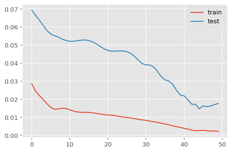 

# Get the predicted values
predictions = model.predict(x_test)
predictions = scaler_pred.inverse_transform(predictions)

1/3 [=========>....................] - ETA: 0s

3/3 [==============================] - ETA: 0s

3/3 [==============================] - 0s 31ms/step

y_test = y_test.reshape(-1,1)
y_test = scaler_pred.inverse_transform(y_test)

# Calculate the mean absolute error (MAE)
mae = mean_absolute_error(y_test, predictions)
print('MAE: ' + str(round(mae, 1)))

# Calculate the root mean squarred error (RMSE)
rmse = np.sqrt(mean_squared_error(y_test,predictions))
print('RMSE: ' + str(round(rmse, 1)))

# Calculate the root mean squarred error (RMSE)
rmse = mean_squared_error(y_test, 
                          predictions,
                          squared = False)
print('RMSE: ' + str(round(rmse, 1)))

MAE: 301.5
RMSE: 408.5
RMSE: 408.5

# Add the difference between the valid and predicted prices
train = data_malaga[:(len(x_train)+92)]
valid = data_malaga[(len(x_train)+91):]

valid.insert(1, "Predictions", predictions, True)
valid.insert(1, "Difference", valid["Predictions"] - valid["num_casos"], True)

# Zoom-in to a closer timeframe
# Date from which on the date is displayed
display_start_date = "2021-07-15" 
valid = valid[valid.index > display_start_date]
train = train[train.index > display_start_date]

# Visualize the data
matplotlib.style.use('ggplot')
fig, ax1 = plt.subplots(figsize=(22, 10), sharex=True)

# Data - Train
xt = train.index; 
yt = train[["num_casos"]]
# Data - Test / validation 
xv = valid.index; 
yv = valid[["num_casos", "Predictions"]]

# Plot
plt.title("malaga: Predictions vs Real infections", fontsize=20)
plt.ylabel("Nº Cases", fontsize=18)

plt.plot(yt, color="blue", linewidth=1.5)
plt.plot(yv["Predictions"], color="red", linewidth=1.5)
plt.plot(yv["num_casos"], color="green", linewidth=1.5)
plt.legend(["Train", "LSTM Predictions", "Test"], 
           loc="upper left", fontsize=18)

# Bar plot with the differences
x = valid.index
y = valid["Difference"]
plt.bar(x, y, width=0.2, color="grey")
plt.grid()
plt.show()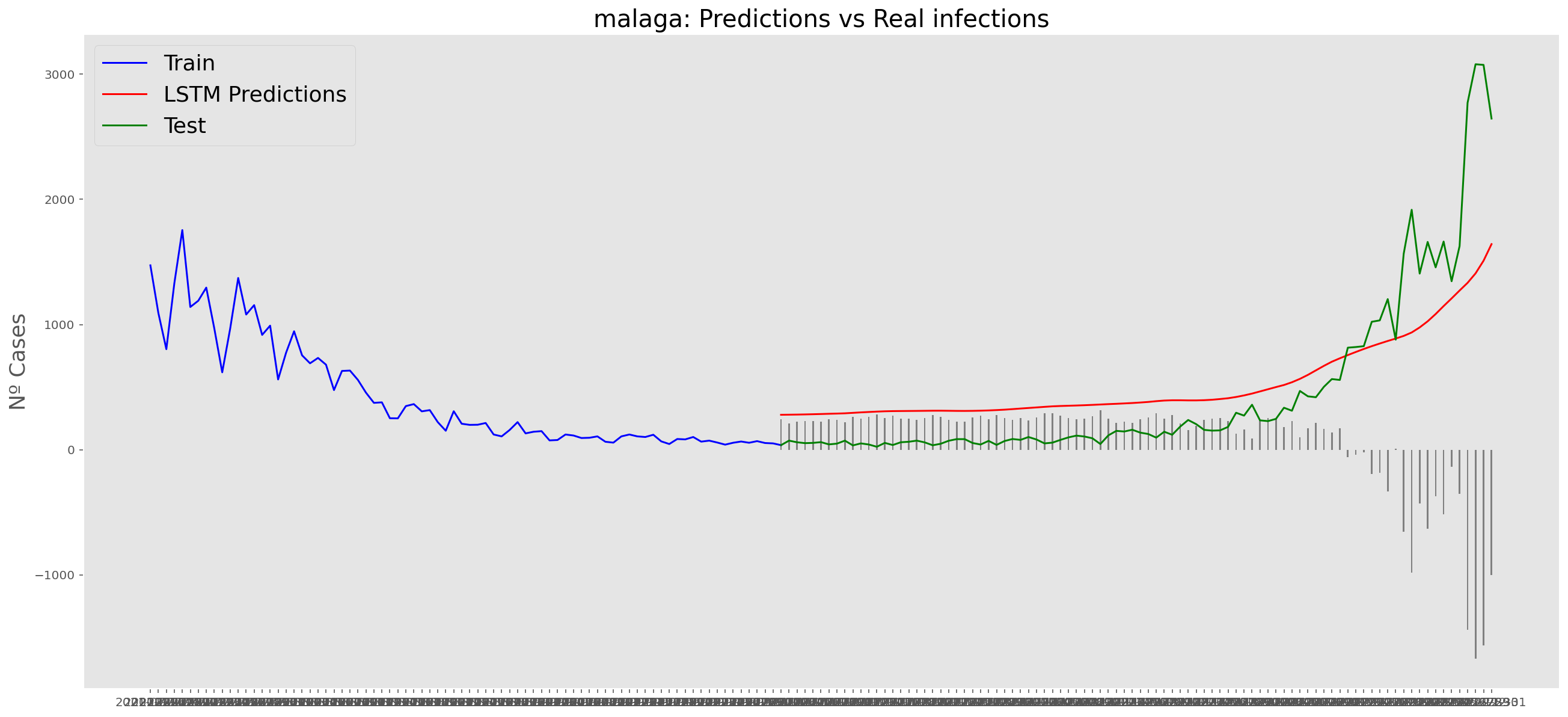

Sevilla

data_sevilla = data_covid.loc[data_covid['provincia'] == 'Sevilla']
data_sevilla = data_sevilla.set_index('fecha')
data_sevilla = data_sevilla['2020-06-14':'2021-12-31']
data_sevilla = data_sevilla.filter(['num_casos', 'tmed', 'mob_grocery_pharmacy', 
'mob_parks', 'mob_residential', 'mob_residential', 'mob_transit_stations', 'mob_workplaces'])
data_sevilla

	num_casos	tmed	mob_grocery_pharmacy	mob_parks	mob_residential	mob_residential	mob_transit_stations	mob_workplaces
fecha
2020-06-14	0	22.200000	-24.0	-36.0	0.0	0.0	-51.0	0.0
2020-06-15	2	23.088889	-14.0	-13.0	9.0	9.0	-41.0	-33.0
2020-06-16	1	23.977778	-10.0	-4.0	9.0	9.0	-37.0	-32.0
2020-06-17	0	24.866667	-10.0	-7.0	9.0	9.0	-37.0	-32.0
2020-06-18	0	25.755556	-12.0	-13.0	9.0	9.0	-41.0	-33.0
...	...	...	...	...	...	...	...	...
2021-12-27	2617	17.600000	16.0	-1.0	7.0	7.0	-19.0	-39.0
2021-12-28	3190	16.000000	17.0	15.0	7.0	7.0	-16.0	-37.0
2021-12-29	3692	14.100000	24.0	18.0	6.0	6.0	-18.0	-38.0
2021-12-30	3508	13.000000	39.0	11.0	6.0	6.0	-21.0	-39.0
2021-12-31	2816	14.600000	15.0	-24.0	12.0	12.0	-44.0	-53.0

566 rows × 8 columns

data_sevilla.describe()

	num_casos	tmed	mob_grocery_pharmacy	mob_parks	mob_residential	mob_residential	mob_transit_stations	mob_workplaces
count	566.000000	566.000000	566.000000	566.000000	566.000000	566.000000	566.000000	566.000000
mean	383.807420	20.691519	-1.908127	-16.176678	4.086572	4.086572	-27.310954	-21.436396
std	454.714408	6.882766	18.249947	18.068323	4.554635	4.554635	14.360299	14.353391
min	0.000000	5.500000	-79.000000	-70.000000	-7.000000	-7.000000	-71.000000	-79.000000
25%	112.750000	15.000000	-10.000000	-28.000000	1.000000	1.000000	-37.000000	-30.000000
50%	260.500000	20.800000	-1.000000	-13.000000	4.000000	4.000000	-28.000000	-18.000000
75%	459.000000	26.575000	6.000000	-5.000000	7.000000	7.000000	-18.000000	-11.000000
max	3692.000000	34.400000	113.000000	61.000000	22.000000	22.000000	16.000000	9.000000

np_data_sevilla = data_sevilla.values

# Train dataset
scaler = MinMaxScaler(feature_range=(0, 1))
scaled_data_sevilla = scaler.fit_transform(np_data_sevilla)
print(f'Longitud del conjunto de datos disponible: {len(scaled_data_sevilla)}')

Longitud del conjunto de datos disponible: 566

# Since we are going to predict future values based on the 90 past elements, 
# we need to create a list with those historic information for each element
historic_values = 90
scaled_data_sevilla_x = []
scaled_data_sevilla_y = []

for i in range(historic_values, len(scaled_data_sevilla)):
    scaled_data_sevilla_x.append(scaled_data_sevilla[(i-historic_values):i, :])
    scaled_data_sevilla_y.append(scaled_data_sevilla[i, 0])

# Convert the x_train and y_train to numpy arrays
scaled_data_sevilla_x = np.array(scaled_data_sevilla_x)
scaled_data_sevilla_y = np.array(scaled_data_sevilla_y)

# Once predicted, we are going to need a exclusive scaler for num_cases
scaler_pred = MinMaxScaler(feature_range=(0, 1))
df_cases_sevilla = pd.DataFrame(data_sevilla['num_casos'])
scaled_data_sevilla_pred = scaler_pred.fit_transform(df_cases_sevilla)

# Since the first 90th values does not have historic, the dataset has been reduced in 90 values
print(f'Longitud datos de entrenamiento con historico: {len(scaled_data_sevilla_y)}')

Longitud datos de entrenamiento con historico: 476

# we split data in train and test
# as in previous analysis, we are going to predict a maximum of 90 days
x_train = scaled_data_sevilla_x[0:len(scaled_data_sevilla_x)-91]
y_train = scaled_data_sevilla_y[0:len(scaled_data_sevilla_y)-91]
print(f'Cantidad datos de entrenamiento: x={len(x_train)} - y={len(y_train)}')

x_test = scaled_data_sevilla_x[len(scaled_data_sevilla_x)-90:len(scaled_data_sevilla_x)]
y_test = scaled_data_sevilla_y[len(scaled_data_sevilla_y)-90:len(scaled_data_sevilla_y)]
print(f'Cantidad datos de test: x={len(x_test)} - y={len(y_test)}')

Cantidad datos de entrenamiento: x=385 - y=385
Cantidad datos de test: x=90 - y=90

# Reshape the data to feed de recurrent network
x_train = np.reshape(x_train, (x_train.shape[0], x_train.shape[1], 8))
print("Train data shape:")
print(x_train.shape)
print(y_train.shape)
x_test = np.reshape(x_test, (x_test.shape[0], x_test.shape[1], 8))
print("Test data shape:")
print(x_test.shape)
print(y_test.shape)

Train data shape:
(385, 90, 8)
(385,)
Test data shape:
(90, 90, 8)
(90,)

# Configure / setup the neural network model - LSTM
# Build the model
print('Build model...')
model = Sequential()
# Model with Neurons 
# Inputshape = neurons -> Timestamps
neurons= x_train.shape[1]
model.add(LSTM(90, 
               activation = 'relu',
               return_sequences = True, 
               input_shape = (x_train.shape[1], 8))) 
model.add(LSTM(50, 
               activation = 'relu',
               return_sequences = True)) 
model.add(LSTM(25, 
               activation = 'relu',
               return_sequences = False)) 
model.add(Dense(5, activation = 'relu'))
model.add(Dense(1))

Build model...

model.compile(optimizer='adam', loss='mean_squared_error')
model.summary()

Model: "sequential_9"

_________________________________________________________________

 Layer (type)                Output Shape              Param #   

=================================================================

 lstm_27 (LSTM)              (None, 90, 90)            35640     

 lstm_28 (LSTM)              (None, 90, 50)            28200     

 lstm_29 (LSTM)              (None, 25)                7600      

 dense_18 (Dense)            (None, 5)                 130       

 dense_19 (Dense)            (None, 1)                 6         

=================================================================

Total params: 71,576

Trainable params: 71,576

Non-trainable params: 0

_________________________________________________________________

# Training the model
# fit network
history = model.fit(x_train, 
                    y_train, 
                    batch_size=1000, 
                    epochs=50, 
                    validation_data = (x_test, y_test), 
                    verbose = 0)

plt.plot(history.history['loss'], label='train')
plt.plot(history.history['val_loss'], label='test')
plt.legend()
plt.show()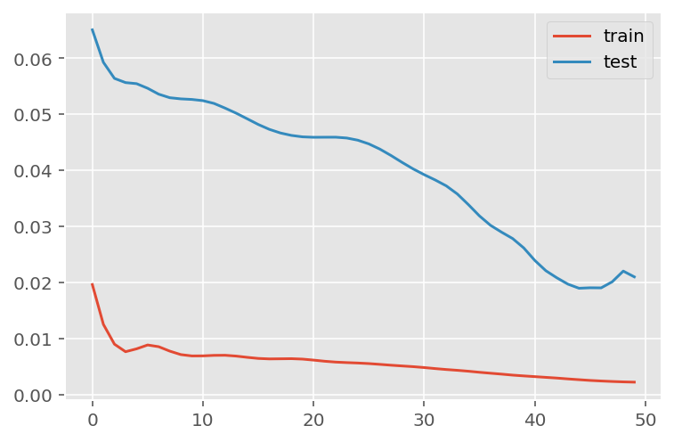 

# Get the predicted values
predictions = model.predict(x_test)
predictions = scaler_pred.inverse_transform(predictions)

1/3 [=========>....................] - ETA: 0s

3/3 [==============================] - ETA: 0s

3/3 [==============================] - 0s 31ms/step

y_test = y_test.reshape(-1,1)
y_test = scaler_pred.inverse_transform(y_test)

# Calculate the mean absolute error (MAE)
mae = mean_absolute_error(y_test, predictions)
print('MAE: ' + str(round(mae, 1)))

# Calculate the root mean squarred error (RMSE)
rmse = np.sqrt(mean_squared_error(y_test,predictions))
print('RMSE: ' + str(round(rmse, 1)))

# Calculate the root mean squarred error (RMSE)
rmse = mean_squared_error(y_test, 
                          predictions,
                          squared = False)
print('RMSE: ' + str(round(rmse, 1)))

MAE: 502.2
RMSE: 535.4
RMSE: 535.4

# Add the difference between the valid and predicted prices
train = data_sevilla[:(len(x_train)+92)]
valid = data_sevilla[(len(x_train)+91):]

valid.insert(1, "Predictions", predictions, True)
valid.insert(1, "Difference", valid["Predictions"] - valid["num_casos"], True)

# Zoom-in to a closer timeframe
# Date from which on the date is displayed
display_start_date = "2021-07-15" 
valid = valid[valid.index > display_start_date]
train = train[train.index > display_start_date]

# Visualize the data
matplotlib.style.use('ggplot')
fig, ax1 = plt.subplots(figsize=(22, 10), sharex=True)

# Data - Train
xt = train.index; 
yt = train[["num_casos"]]
# Data - Test / validation 
xv = valid.index; 
yv = valid[["num_casos", "Predictions"]]

# Plot
plt.title("sevilla: Predictions vs Real infections", fontsize=20)
plt.ylabel("Nº Cases", fontsize=18)

plt.plot(yt, color="blue", linewidth=1.5)
plt.plot(yv["Predictions"], color="red", linewidth=1.5)
plt.plot(yv["num_casos"], color="green", linewidth=1.5)
plt.legend(["Train", "LSTM Predictions", "Test"], 
           loc="upper left", fontsize=18)

# Bar plot with the differences
x = valid.index
y = valid["Difference"]
plt.bar(x, y, width=0.2, color="grey")
plt.grid()
plt.show()