pacman::p_load(
      here,      # file locator
      tidyverse, # data management and ggplot2 graphics
      skimr,     # get overview of data
      janitor,   # produce and adorn tabulations and cross-tabulations
      tsibble,
      fable,
      feasts,
      fabletools,
      lubridate
)

covid_data <- readRDS(here("data", "clean", "final_covid_data.rds"))Univariate prediction
Load packages:
For each period to study, we will train three different models:
- Attempt 1: using ARIMA function from fable package with stepwise (much faster)
- Attempt 2: using ARIMA function from fable package without stepwise
- Attempt 3: using Snaive function from fable package
Before sixth epidemiological period
On one hand, we are going to train the model with data previous the start of the sixth wave of coronavirus (14 oct 2021).
On the other hand, we are going to train the model with data as of June 14th which is considered the beginning of the second epidemiological period in Spain.
Asturias
data_asturias <- covid_data %>%
      filter(provincia == "Asturias") %>%
      filter(fecha > as.Date("2020-06-14", format = "%Y-%m-%d")) %>%
      select(provincia, fecha, num_casos, num_hosp, tmed,mob_grocery_pharmacy, mob_parks,
             mob_residential, mob_retail_recreation, mob_transit_stations, mob_workplaces, mob_flujo) %>%
      drop_na(-mob_flujo) %>%
      as_tsibble(key = provincia, index = fecha)
data_asturias
# A tsibble: 653 x 12 [1D]
# Key: provincia [1]
provincia fecha num_casos num_hosp tmed mob_grocery_pharmacy mob_parks
<chr> <date> <dbl> <dbl> <dbl> <dbl> <dbl>
1 Asturias 2020-06-15 0 0 16 -6 39
2 Asturias 2020-06-16 1 0 15.6 -6 7
3 Asturias 2020-06-17 0 0 15.6 -7 20
4 Asturias 2020-06-18 0 0 15.1 -4 68
5 Asturias 2020-06-19 0 0 14.8 -4 52
6 Asturias 2020-06-20 0 0 16.8 -10 71
7 Asturias 2020-06-21 0 0 18.2 -5.5 46
8 Asturias 2020-06-22 0 0 18.2 -1 99
9 Asturias 2020-06-23 0 0 20 -2 129
10 Asturias 2020-06-24 0 0 18.2 -9 63
# … with 643 more rows, and 5 more variables: mob_residential <dbl>,
# mob_retail_recreation <dbl>, mob_transit_stations <dbl>,
# mob_workplaces <dbl>, mob_flujo <dbl>data_asturias_train <- data_asturias %>%
filter(fecha <= as.Date("2021-10-14", format = "%Y-%m-%d"))
summary(data_asturias_train$fecha) Min. 1st Qu. Median Mean 3rd Qu. Max.
"2020-06-15" "2020-10-14" "2021-02-13" "2021-02-13" "2021-06-14" "2021-10-14" data_asturias_test <- data_asturias %>%
filter(fecha > as.Date("2021-10-14", format = "%Y-%m-%d"))
summary(data_asturias_test$fecha) Min. 1st Qu. Median Mean 3rd Qu. Max.
"2021-10-15" "2021-11-25" "2022-01-05" "2022-01-05" "2022-02-15" "2022-03-29" lambda_asturias <- data_asturias %>%
features(num_casos, features = guerrero) %>%
pull(lambda_guerrero)
fit_model <- data_asturias_train %>%
model(
arima_at1 = ARIMA(box_cox(num_casos, lambda_asturias)),
arima_at2 = ARIMA(box_cox(num_casos, lambda_asturias),
stepwise = FALSE, approx = FALSE),
Snaive = SNAIVE(box_cox(num_casos, lambda_asturias))
)
# Show and report model
fit_model# A mable: 1 x 4
# Key: provincia [1]
provincia arima_at1 arima_at2 Snaive
<chr> <model> <model> <model>
1 Asturias <ARIMA(3,1,1)(2,0,0)[7]> <ARIMA(2,1,4)> <SNAIVE>glance(fit_model)# A tibble: 3 × 9
provincia .model sigma2 log_lik AIC AICc BIC ar_roots ma_roots
<chr> <chr> <dbl> <dbl> <dbl> <dbl> <dbl> <list> <list>
1 Asturias arima_at1 0.944 -673. 1360. 1360. 1390. <cpl [17]> <cpl [1]>
2 Asturias arima_at2 0.910 -664. 1343. 1343. 1372. <cpl [2]> <cpl [4]>
3 Asturias Snaive 2.32 NA NA NA NA <NULL> <NULL> fit_model %>%
pivot_longer(-provincia,
names_to = ".model",
values_to = "orders") %>%
left_join(glance(fit_model), by = c("provincia", ".model")) %>%
arrange(AICc) %>%
select(.model:BIC)# A mable: 3 x 7
# Key: .model [3]
.model orders sigma2 log_lik AIC AICc BIC
<chr> <model> <dbl> <dbl> <dbl> <dbl> <dbl>
1 arima_at2 <ARIMA(2,1,4)> 0.910 -664. 1343. 1343. 1372.
2 arima_at1 <ARIMA(3,1,1)(2,0,0)[7]> 0.944 -673. 1360. 1360. 1390.
3 Snaive <SNAIVE> 2.32 NA NA NA NA # We use a Ljung-Box test >> large p-value, confirms residuals are similar / considered to white noise
fit_model %>%
select(Snaive) %>%
gg_tsresiduals()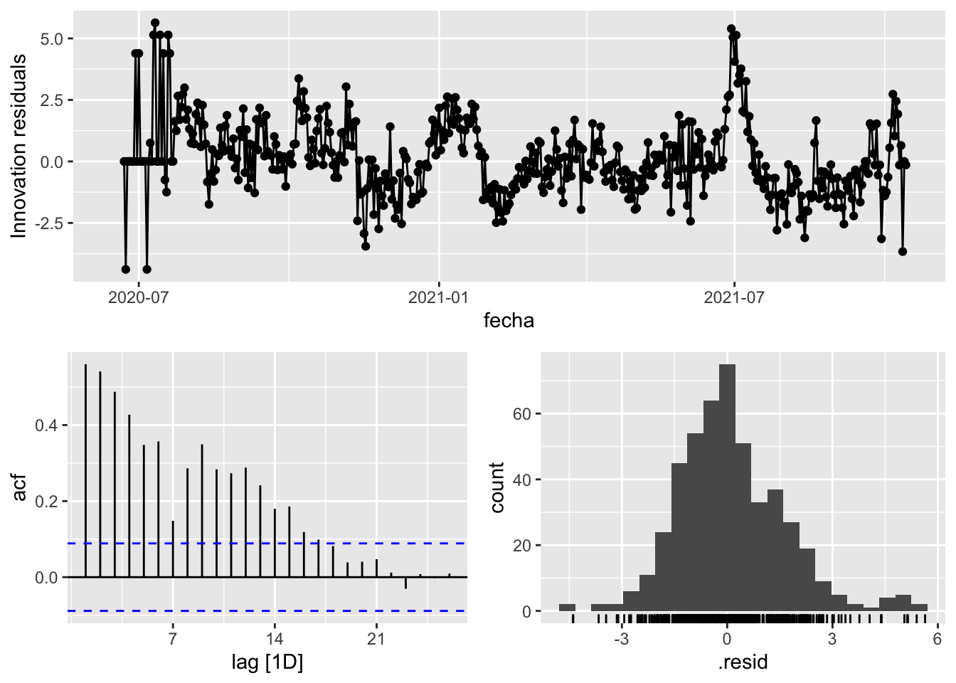
fit_model %>%
      select(arima_at1) %>%
      gg_tsresiduals()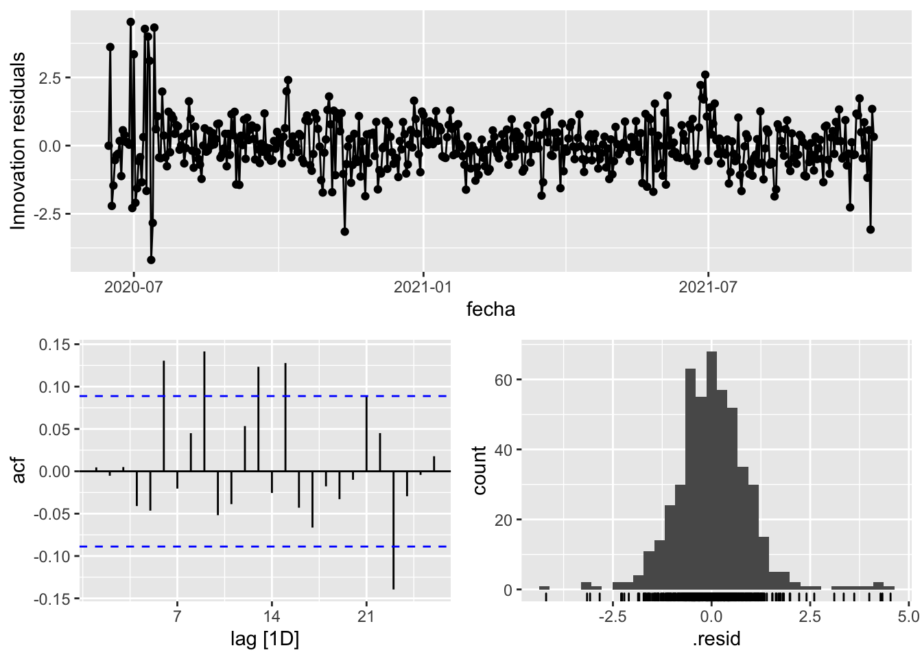
fit_model %>%
      select(arima_at2) %>%
      gg_tsresiduals()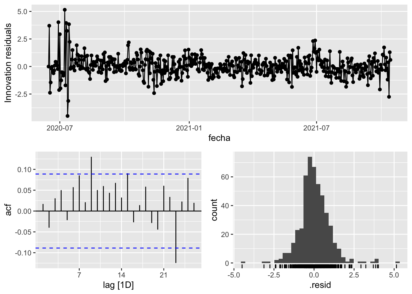
augment(fit_model) %>%
      features(.innov, ljung_box, lag=7)
# A tibble: 3 × 4
provincia .model lb_stat lb_pvalue
<chr> <chr> <dbl> <dbl>
1 Asturias arima_at1 10.6 0.158
2 Asturias arima_at2 8.11 0.323
3 Asturias Snaive 629. 0 augment(fit_model) %>%
features(.innov, ljung_box, lag=14)# A tibble: 3 × 4
provincia .model lb_stat lb_pvalue
<chr> <chr> <dbl> <dbl>
1 Asturias arima_at1 33.1 0.00282
2 Asturias arima_at2 23.6 0.0509
3 Asturias Snaive 892. 0 augment(fit_model) %>%
features(.innov, ljung_box, lag=21)# A tibble: 3 × 4
provincia .model lb_stat lb_pvalue
<chr> <chr> <dbl> <dbl>
1 Asturias arima_at1 49.3 0.000460
2 Asturias arima_at2 33.3 0.0433
3 Asturias Snaive 927. 0 augment(fit_model) %>%
features(.innov, ljung_box, lag=90)# A tibble: 3 × 4
provincia .model lb_stat lb_pvalue
<chr> <chr> <dbl> <dbl>
1 Asturias arima_at1 118. 0.0242
2 Asturias arima_at2 86.5 0.584
3 Asturias Snaive 1195. 0 # Significant spikes out of 30 is still consistent with white noise
# To be sure, use a Ljung-Box test, which has a large p-value, confirming that
# the residuals are similar to white noise.
# Note that the alternative models also passed this test.
#
# Forecast
fc_h7 <- fabletools::forecast(fit_model, h = 7)
fc_h14 <- fabletools::forecast(fit_model, h = 14)
fc_h21 <- fabletools::forecast(fit_model, h = 21)
fc_h90 <- fabletools::forecast(fit_model, h = 90)7 days
# Plots
fc_h7 %>%
      autoplot(
            data_asturias_test %>%
                  filter(fecha <= as.Date("2021-10-14", format = "%Y-%m-%d")+days(9))
      ) +
      labs(y = "Nº cases", title = "Asturias - forecast h7")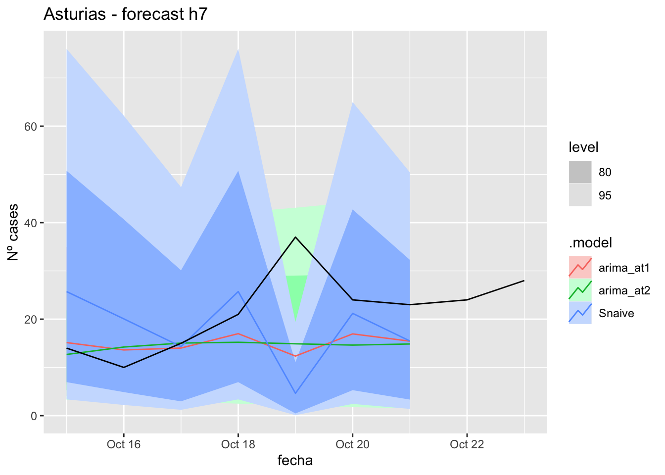
fc_h7 %>%
      autoplot(
            data_asturias %>%
                  filter(fecha <= as.Date("2021-10-14", format = "%Y-%m-%d")+days(9) &
                               fecha > as.Date("2021-07-01", format = "%Y-%m-%d"))
      ) +
      labs(y = "Nº cases", title = "Asturias - forecast h7")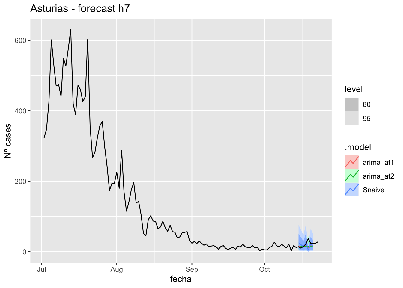
# Accuracy
fabletools::accuracy(fc_h7, data_asturias)
# A tibble: 3 × 11
.model provincia .type ME RMSE MAE MPE MAPE MASE RMSSE ACF1
<chr> <chr> <chr> <dbl> <dbl> <dbl> <dbl> <dbl> <dbl> <dbl> <dbl>
1 arima_at1 Asturias Test 5.64 10.3 7.00 15.7 28.4 0.141 0.126 0.214
2 arima_at2 Asturias Test 6.06 9.97 7.28 18.4 30.5 0.147 0.121 0.385
3 Snaive Asturias Test 2.41 14.0 9.98 -10.1 49.0 0.201 0.171 0.0076614 days
# Plots
fc_h14 %>%
      autoplot(
            data_asturias_test %>%
                  filter(fecha <= as.Date("2021-10-14", format = "%Y-%m-%d")+days(16))
      ) +
      labs(y = "Nº cases", title = "Asturias - forecast h14")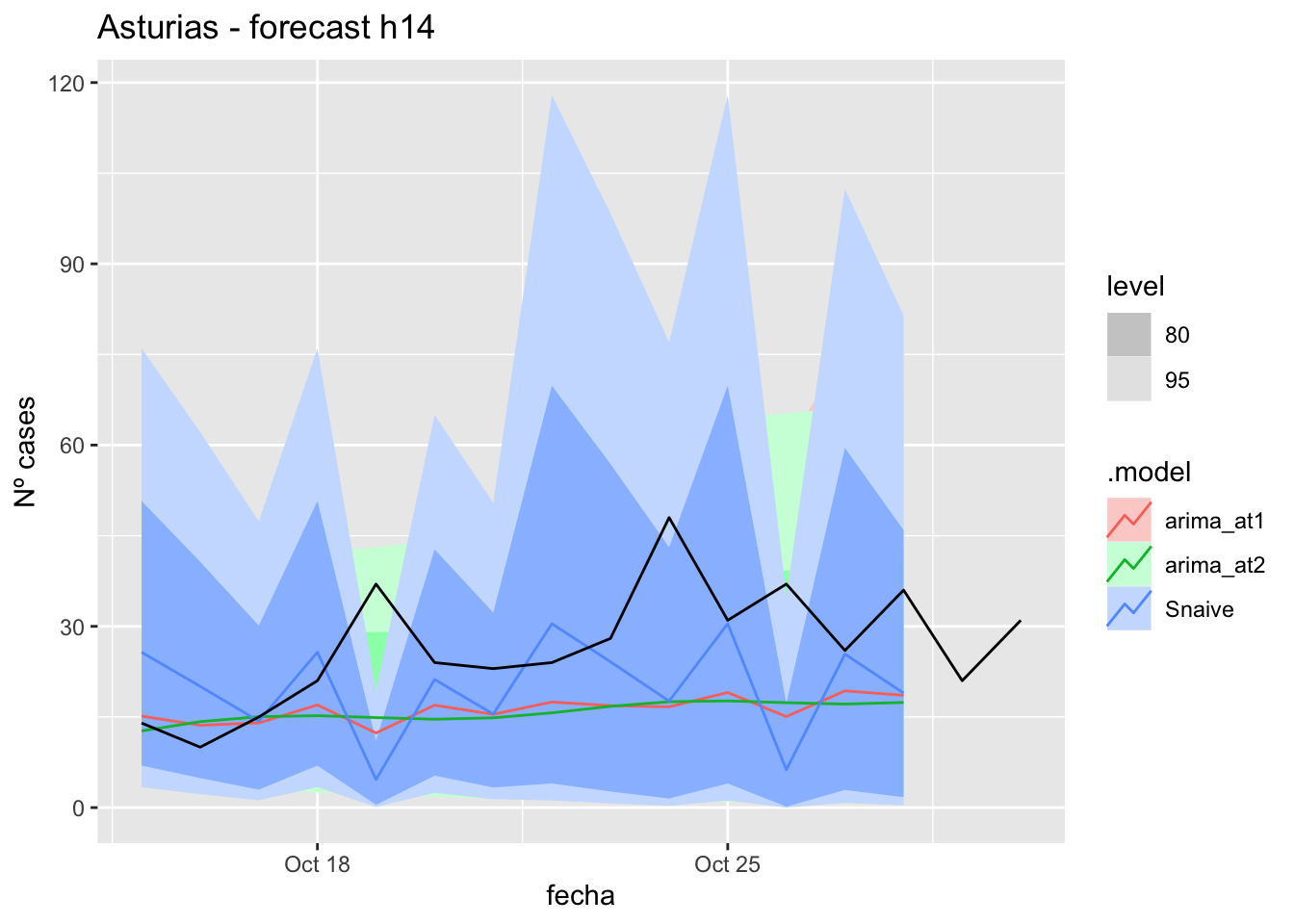
fc_h14 %>%
      autoplot(
            data_asturias %>%
                  filter(fecha <= as.Date("2021-10-14", format = "%Y-%m-%d")+days(16) &
                               fecha > as.Date("2021-07-01", format = "%Y-%m-%d"))
      ) +
      labs(y = "Nº cases", title = "Asturias - forecast h14")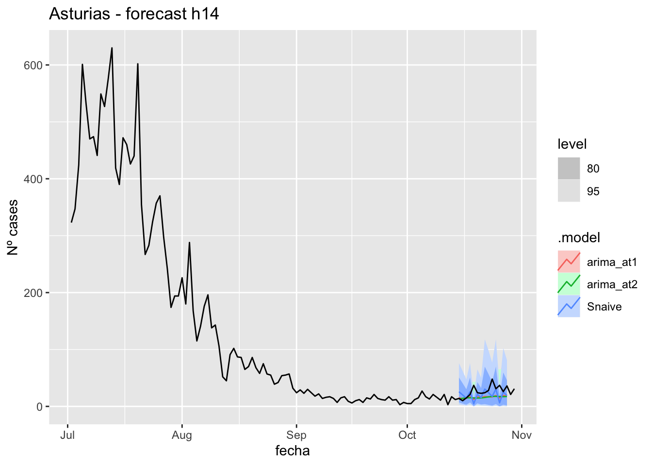
# Accuracy
fabletools::accuracy(fc_h14, data_asturias)
# A tibble: 3 × 11
.model provincia .type ME RMSE MAE MPE MAPE MASE RMSSE ACF1
<chr> <chr> <chr> <dbl> <dbl> <dbl> <dbl> <dbl> <dbl> <dbl> <dbl>
1 arima_at1 Asturias Test 10.5 14.3 11.1 29.6 35.9 0.224 0.174 0.172
2 arima_at2 Asturias Test 10.9 14.2 11.5 32.1 38.1 0.232 0.173 0.303
3 Snaive Asturias Test 6.69 16.0 11.4 8.17 41.5 0.229 0.195 -0.15621 days
# Plots
fc_h21 %>%
      autoplot(
            data_asturias_test %>%
                  filter(fecha <= as.Date("2021-10-14", format = "%Y-%m-%d")+days(23))
      ) +
      labs(y = "Nº cases", title = "Asturias - forecast h21")
fc_h21 %>%
      autoplot(
            data_asturias %>%
                  filter(fecha <= as.Date("2021-10-14", format = "%Y-%m-%d")+days(23) &
                               fecha > as.Date("2021-07-01", format = "%Y-%m-%d"))
      ) +
      labs(y = "Nº cases", title = "Asturias - forecast h21")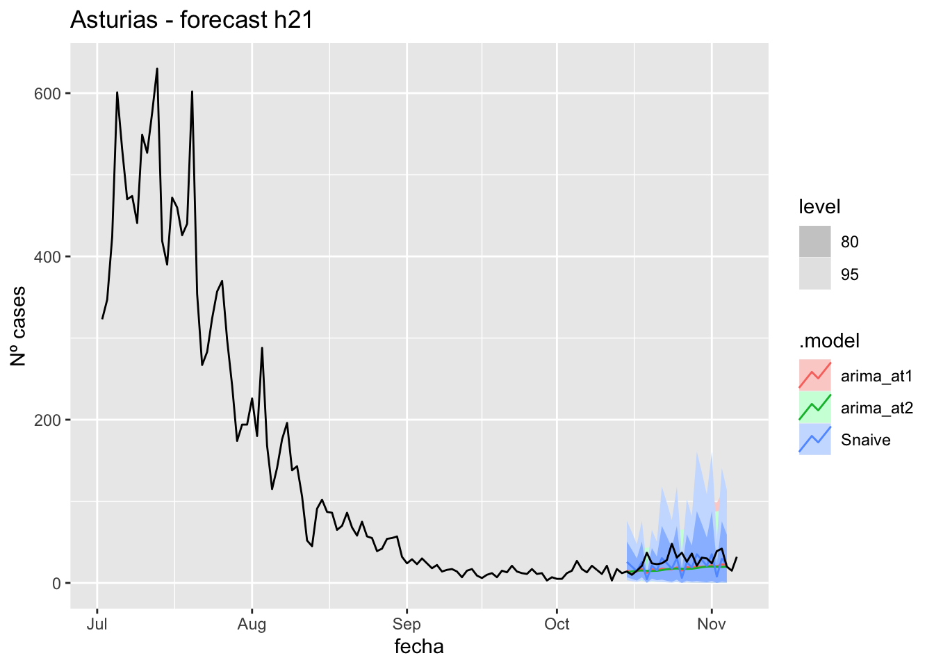
# Accuracy
fabletools::accuracy(fc_h21, data_asturias)
# A tibble: 3 × 11
.model provincia .type ME RMSE MAE MPE MAPE MASE RMSSE ACF1
<chr> <chr> <chr> <dbl> <dbl> <dbl> <dbl> <dbl> <dbl> <dbl> <dbl>
1 arima_at1 Asturias Test 9.79 13.5 10.5 27.5 32.9 0.211 0.164 0.0331
2 arima_at2 Asturias Test 10.6 13.7 11.0 31.0 35.1 0.222 0.167 0.126
3 Snaive Asturias Test 5.77 15.6 11.5 6.52 40.8 0.232 0.190 -0.223 90 days
# Plots
fc_h90 %>%
      autoplot(
            data_asturias_test %>%
                  filter(fecha <= as.Date("2021-10-14", format = "%Y-%m-%d")+days(92))
      ) +
      labs(y = "Nº cases", title = "Asturias - forecast h90")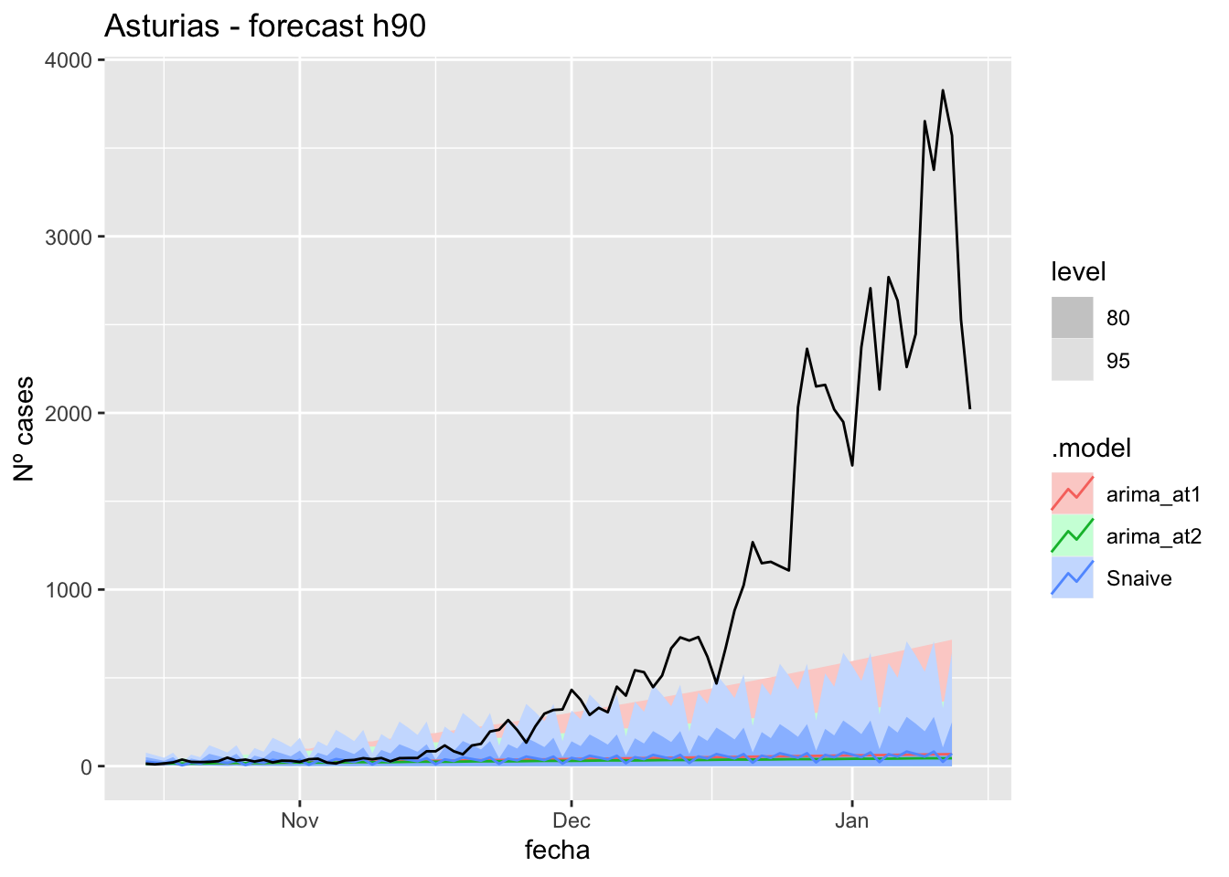
fc_h90 %>%
      autoplot(
            data_asturias %>%
                  filter(fecha <= as.Date("2021-10-14", format = "%Y-%m-%d")+days(92) &
                               fecha > as.Date("2021-07-01", format = "%Y-%m-%d"))
      ) +
      labs(y = "Nº cases", title = "Asturias - forecast h90")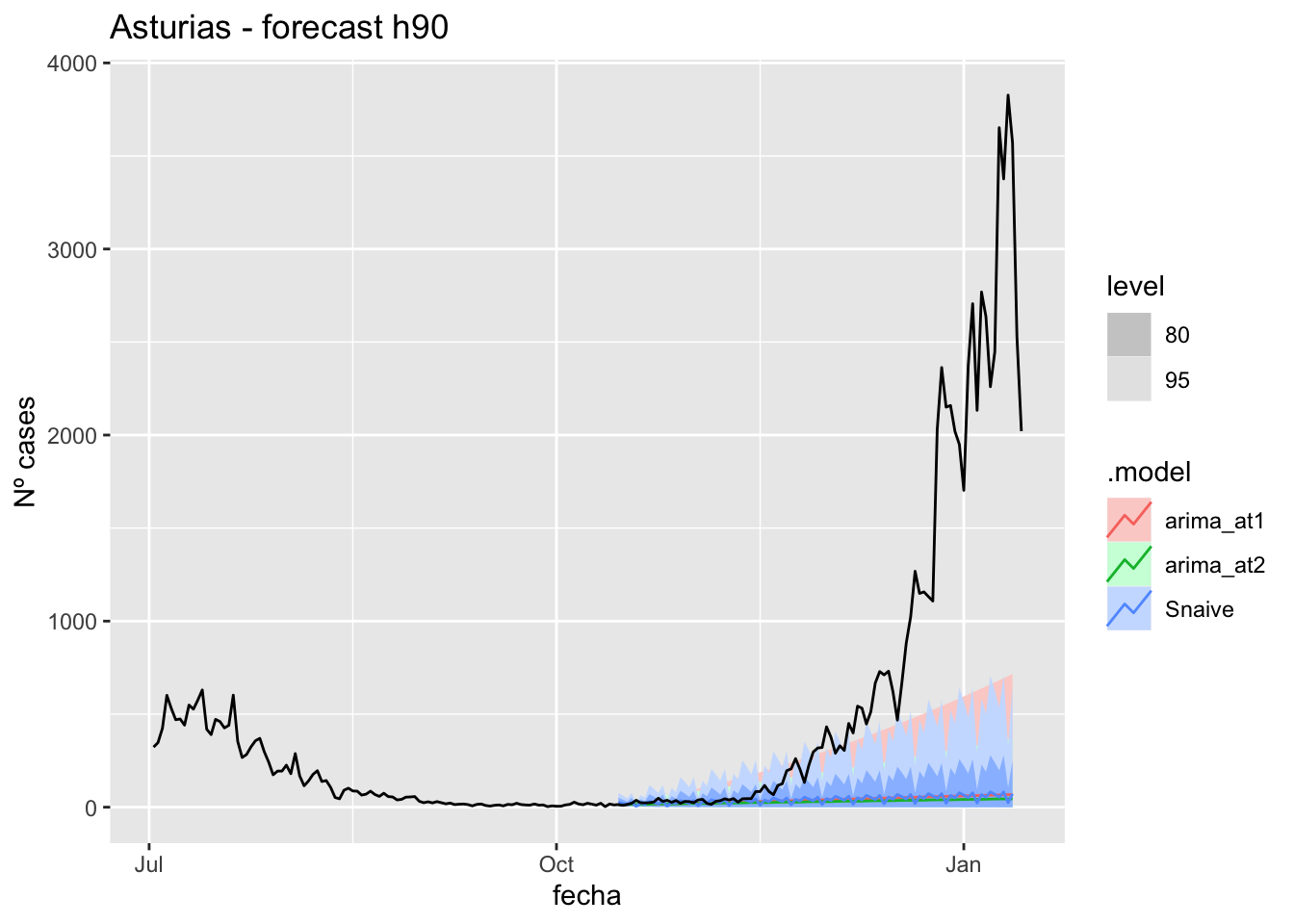
# Accuracy
fabletools::accuracy(fc_h90, data_asturias)
# A tibble: 3 × 11
.model provincia .type ME RMSE MAE MPE MAPE MASE RMSSE ACF1
<chr> <chr> <chr> <dbl> <dbl> <dbl> <dbl> <dbl> <dbl> <dbl> <dbl>
1 arima_at1 Asturias Test 704. 1211. 704. 67.5 70.0 14.2 14.8 0.925
2 arima_at2 Asturias Test 713. 1221. 714. 71.1 72.9 14.4 14.9 0.926
3 Snaive Asturias Test 702. 1213. 704. 60.0 71.7 14.2 14.8 0.925Barcelona
data_barcelona <- covid_data %>%
      filter(provincia == "Barcelona") %>%
      filter(fecha > as.Date("2020-06-14", format = "%Y-%m-%d")) %>%
      select(provincia, fecha, num_casos, num_hosp, tmed,mob_grocery_pharmacy, mob_parks,
             mob_residential, mob_retail_recreation, mob_transit_stations, mob_workplaces, mob_flujo) %>%
      drop_na(-mob_flujo) %>%
      as_tsibble(key = provincia, index = fecha)
data_barcelona
# A tsibble: 653 x 12 [1D]
# Key: provincia [1]
provincia fecha num_casos num_hosp tmed mob_grocery_pharmacy mob_parks
<chr> <date> <dbl> <dbl> <dbl> <dbl> <dbl>
1 Barcelona 2020-06-15 62 3 21.2 -9 17
2 Barcelona 2020-06-16 66 3 20.8 -10 -16
3 Barcelona 2020-06-17 70 4 20.3 -4 14
4 Barcelona 2020-06-18 68 4 18.8 -8 -6
5 Barcelona 2020-06-19 65 4 20.4 -5 10
6 Barcelona 2020-06-20 53 4 21.8 -12 15
7 Barcelona 2020-06-21 38 1 22.8 -18 18
8 Barcelona 2020-06-22 69 5 23.8 5 24
9 Barcelona 2020-06-23 95 3 23.4 19 28
10 Barcelona 2020-06-24 44 4 23.6 -71 28
# … with 643 more rows, and 5 more variables: mob_residential <dbl>,
# mob_retail_recreation <dbl>, mob_transit_stations <dbl>,
# mob_workplaces <dbl>, mob_flujo <dbl>data_barcelona_train <- data_barcelona %>%
filter(fecha <= as.Date("2021-10-14", format = "%Y-%m-%d"))
summary(data_barcelona_train$fecha) Min. 1st Qu. Median Mean 3rd Qu. Max.
"2020-06-15" "2020-10-14" "2021-02-13" "2021-02-13" "2021-06-14" "2021-10-14" data_barcelona_test <- data_barcelona %>%
filter(fecha > as.Date("2021-10-14", format = "%Y-%m-%d"))
summary(data_barcelona_test$fecha) Min. 1st Qu. Median Mean 3rd Qu. Max.
"2021-10-15" "2021-11-25" "2022-01-05" "2022-01-05" "2022-02-15" "2022-03-29" lambda_Barcelona <- data_barcelona %>%
features(num_casos, features = guerrero) %>%
pull(lambda_guerrero)
fit_model <- data_barcelona_train %>%
model(
arima_at1 = ARIMA(box_cox(num_casos, lambda_Barcelona)),
arima_at2 = ARIMA(box_cox(num_casos, lambda_Barcelona),
stepwise = FALSE, approx = FALSE),
Snaive = SNAIVE(box_cox(num_casos, lambda_Barcelona))
)
# Show and report model
fit_model# A mable: 1 x 4
# Key: provincia [1]
provincia arima_at1 arima_at2 Snaive
<chr> <model> <model> <model>
1 Barcelona <ARIMA(0,1,3)(0,1,2)[7]> <ARIMA(1,1,2)(0,1,2)[7]> <SNAIVE>glance(fit_model)# A tibble: 3 × 9
provincia .model sigma2 log_lik AIC AICc BIC ar_roots ma_roots
<chr> <chr> <dbl> <dbl> <dbl> <dbl> <dbl> <list> <list>
1 Barcelona arima_at1 0.196 -293. 597. 598. 622. <cpl [0]> <cpl [17]>
2 Barcelona arima_at2 0.188 -283. 579. 579. 604. <cpl [1]> <cpl [16]>
3 Barcelona Snaive 0.964 NA NA NA NA <NULL> <NULL> fit_model %>%
pivot_longer(-provincia,
names_to = ".model",
values_to = "orders") %>%
left_join(glance(fit_model), by = c("provincia", ".model")) %>%
arrange(AICc) %>%
select(.model:BIC)# A mable: 3 x 7
# Key: .model [3]
.model orders sigma2 log_lik AIC AICc BIC
<chr> <model> <dbl> <dbl> <dbl> <dbl> <dbl>
1 arima_at2 <ARIMA(1,1,2)(0,1,2)[7]> 0.188 -283. 579. 579. 604.
2 arima_at1 <ARIMA(0,1,3)(0,1,2)[7]> 0.196 -293. 597. 598. 622.
3 Snaive <SNAIVE> 0.964 NA NA NA NA # We use a Ljung-Box test >> large p-value, confirms residuals are similar / considered to white noise
fit_model %>%
select(Snaive) %>%
gg_tsresiduals()
fit_model %>%
      select(arima_at1) %>%
      gg_tsresiduals()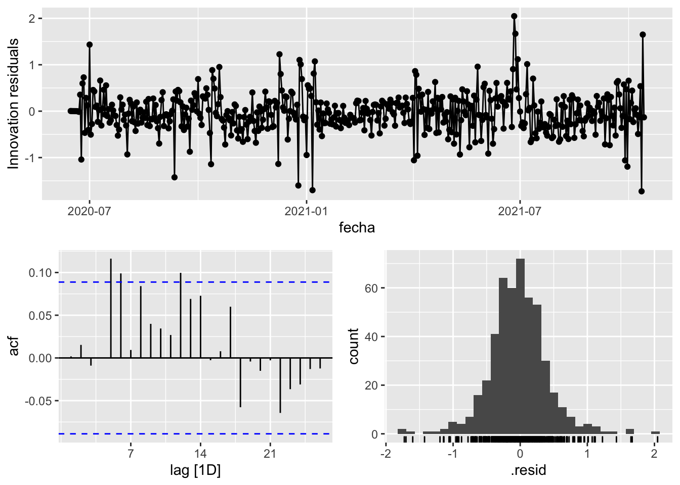
fit_model %>%
      select(arima_at2) %>%
      gg_tsresiduals()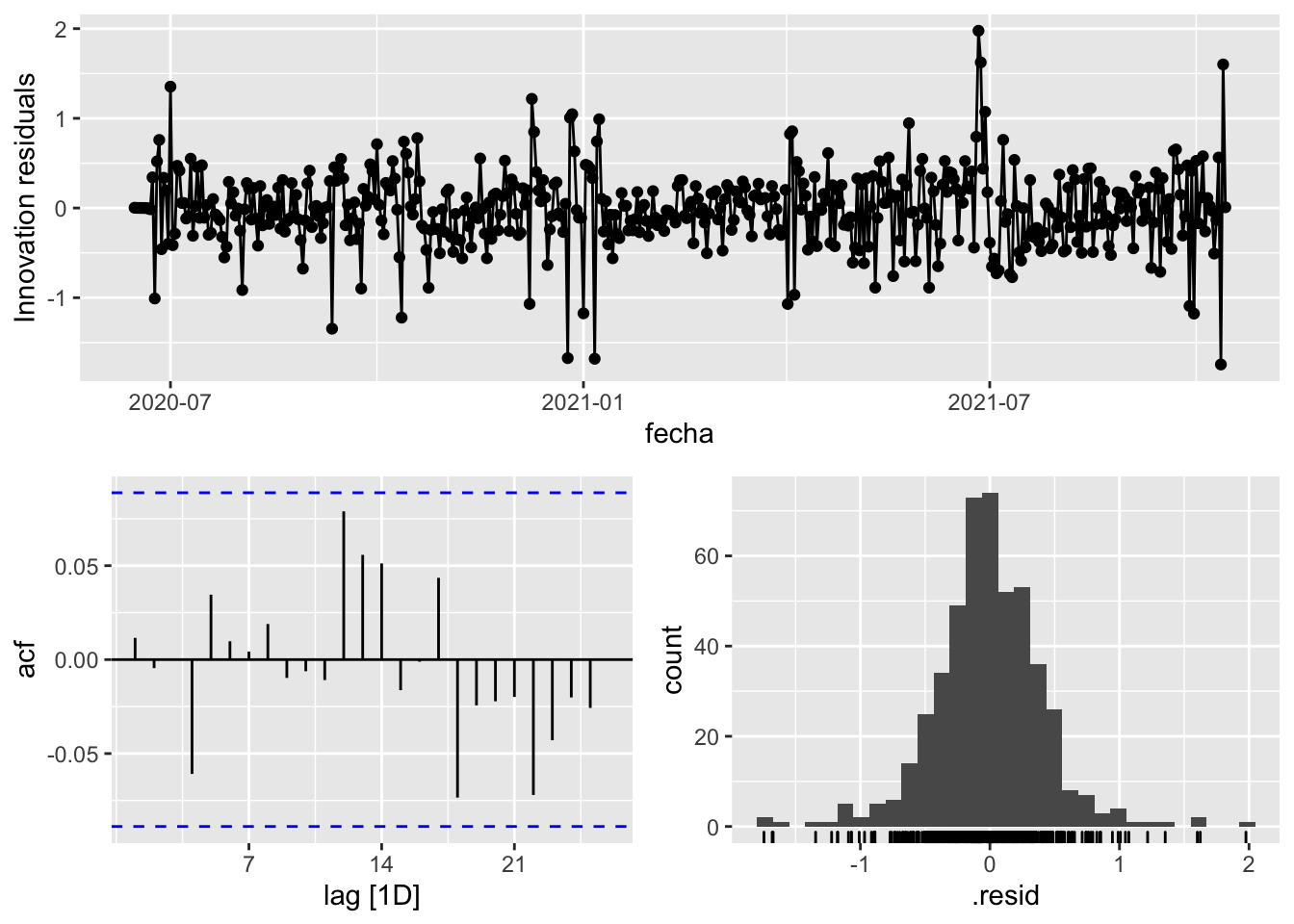
augment(fit_model) %>%
      features(.innov, ljung_box, lag=7)
# A tibble: 3 × 4
provincia .model lb_stat lb_pvalue
<chr> <chr> <dbl> <dbl>
1 Barcelona arima_at1 11.7 0.110
2 Barcelona arima_at2 2.55 0.923
3 Barcelona Snaive 1610. 0 augment(fit_model) %>%
features(.innov, ljung_box, lag=14)# A tibble: 3 × 4
provincia .model lb_stat lb_pvalue
<chr> <chr> <dbl> <dbl>
1 Barcelona arima_at1 27.0 0.0191
2 Barcelona arima_at2 8.86 0.840
3 Barcelona Snaive 2198. 0 augment(fit_model) %>%
features(.innov, ljung_box, lag=21)# A tibble: 3 × 4
provincia .model lb_stat lb_pvalue
<chr> <chr> <dbl> <dbl>
1 Barcelona arima_at1 30.7 0.0788
2 Barcelona arima_at2 13.4 0.892
3 Barcelona Snaive 2259. 0 augment(fit_model) %>%
features(.innov, ljung_box, lag=90)# A tibble: 3 × 4
provincia .model lb_stat lb_pvalue
<chr> <chr> <dbl> <dbl>
1 Barcelona arima_at1 131. 0.00328
2 Barcelona arima_at2 88.9 0.513
3 Barcelona Snaive 3453. 0 # Significant spikes out of 30 is still consistent with white noise
# To be sure, use a Ljung-Box test, which has a large p-value, confirming that
# the residuals are similar to white noise.
# Note that the alternative models also passed this test.
#
# Forecast
fc_h7 <- fabletools::forecast(fit_model, h = 7)
fc_h14 <- fabletools::forecast(fit_model, h = 14)
fc_h21 <- fabletools::forecast(fit_model, h = 21)
fc_h90 <- fabletools::forecast(fit_model, h = 90)7 days
# Plots
fc_h7 %>%
      autoplot(
            data_barcelona_test %>%
                  filter(fecha <= as.Date("2021-10-14", format = "%Y-%m-%d")+days(9))
      ) +
      labs(y = "Nº cases", title = "Barcelona - forecast h7")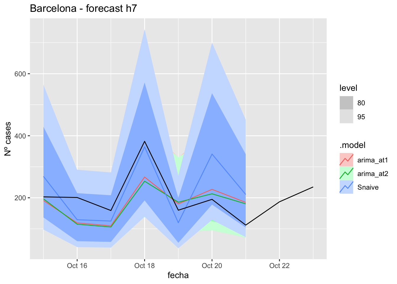
fc_h7 %>%
      autoplot(
            data_barcelona %>%
                  filter(fecha <= as.Date("2021-10-14", format = "%Y-%m-%d")+days(9) &
                               fecha > as.Date("2021-07-01", format = "%Y-%m-%d"))
      ) +
      labs(y = "Nº cases", title = "Barcelona - forecast h7")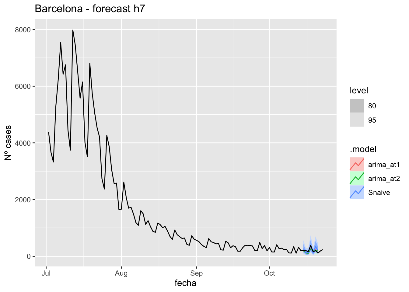
# Accuracy
fabletools::accuracy(fc_h7, data_barcelona)
# A tibble: 3 × 11
.model provincia .type ME RMSE MAE MPE MAPE MASE RMSSE ACF1
<chr> <chr> <chr> <dbl> <dbl> <dbl> <dbl> <dbl> <dbl> <dbl> <dbl>
1 arima_at1 Barcelona Test 18.9 64.7 54.8 1.87 28.9 0.146 0.0976 0.273
2 arima_at2 Barcelona Test 23.0 68.1 55.2 3.74 28.5 0.147 0.103 0.160
3 Snaive Barcelona Test -21.0 79.0 67.8 -15.5 40.3 0.180 0.119 0.18414 days
# Plots
fc_h14 %>%
      autoplot(
            data_barcelona_test %>%
                  filter(fecha <= as.Date("2021-10-14", format = "%Y-%m-%d")+days(16))
      ) +
      labs(y = "Nº cases", title = "Barcelona - forecast h14")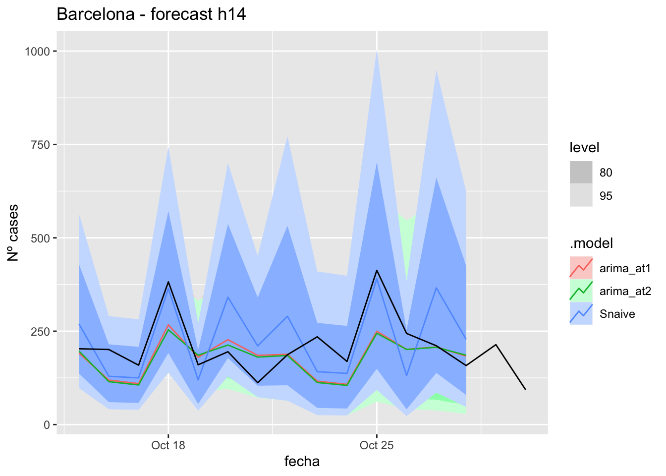
fc_h14 %>%
      autoplot(
            data_barcelona %>%
                  filter(fecha <= as.Date("2021-10-14", format = "%Y-%m-%d")+days(16) &
                               fecha > as.Date("2021-07-01", format = "%Y-%m-%d"))
      ) +
      labs(y = "Nº cases", title = "Barcelona - forecast h14")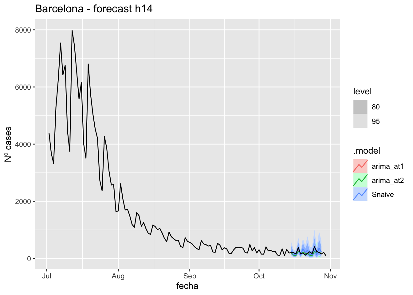
# Accuracy
fabletools::accuracy(fc_h14, data_barcelona)
# A tibble: 3 × 11
.model provincia .type ME RMSE MAE MPE MAPE MASE RMSSE ACF1
<chr> <chr> <chr> <dbl> <dbl> <dbl> <dbl> <dbl> <dbl> <dbl> <dbl>
1 arima_at1 Barcelona Test 35.3 73.8 57.1 10.1 26.0 0.152 0.111 0.279
2 arima_at2 Barcelona Test 38.4 76.8 58.4 11.4 26.3 0.155 0.116 0.216
3 Snaive Barcelona Test -15.3 87.1 76.0 -12.2 40.4 0.202 0.131 0.061021 days
# Plots
fc_h21 %>%
      autoplot(
            data_barcelona_test %>%
                  filter(fecha <= as.Date("2021-10-14", format = "%Y-%m-%d")+days(23))
      ) +
      labs(y = "Nº cases", title = "Barcelona - forecast h21")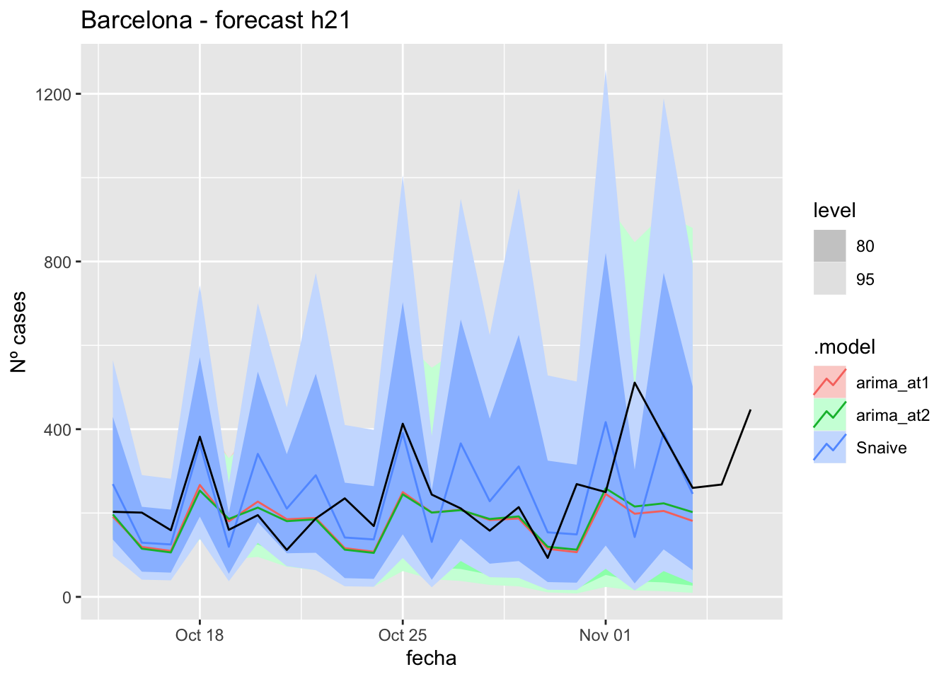
fc_h21 %>%
      autoplot(
            data_barcelona %>%
                  filter(fecha <= as.Date("2021-10-14", format = "%Y-%m-%d")+days(23) &
                               fecha > as.Date("2021-07-01", format = "%Y-%m-%d"))
      ) +
      labs(y = "Nº cases", title = "Barcelona - forecast h21")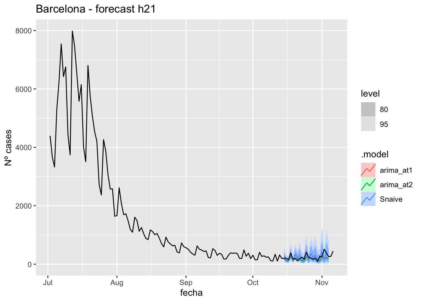
# Accuracy
fabletools::accuracy(fc_h21, data_barcelona)
# A tibble: 3 × 11
.model provincia .type ME RMSE MAE MPE MAPE MASE RMSSE ACF1
<chr> <chr> <chr> <dbl> <dbl> <dbl> <dbl> <dbl> <dbl> <dbl> <dbl>
1 arima_at1 Barcelona Test 58.9 107. 75.5 15.8 28.6 0.201 0.161 0.191
2 arima_at2 Barcelona Test 56.9 103. 73.6 15.2 28.1 0.196 0.156 0.104
3 Snaive Barcelona Test -2.10 119. 90.4 -10.9 41.3 0.240 0.179 -0.23990 days
# Plots
fc_h90 %>%
      autoplot(
            data_barcelona_test %>%
                  filter(fecha <= as.Date("2021-10-14", format = "%Y-%m-%d")+days(92))
      ) +
      labs(y = "Nº cases", title = "Barcelona - forecast h90")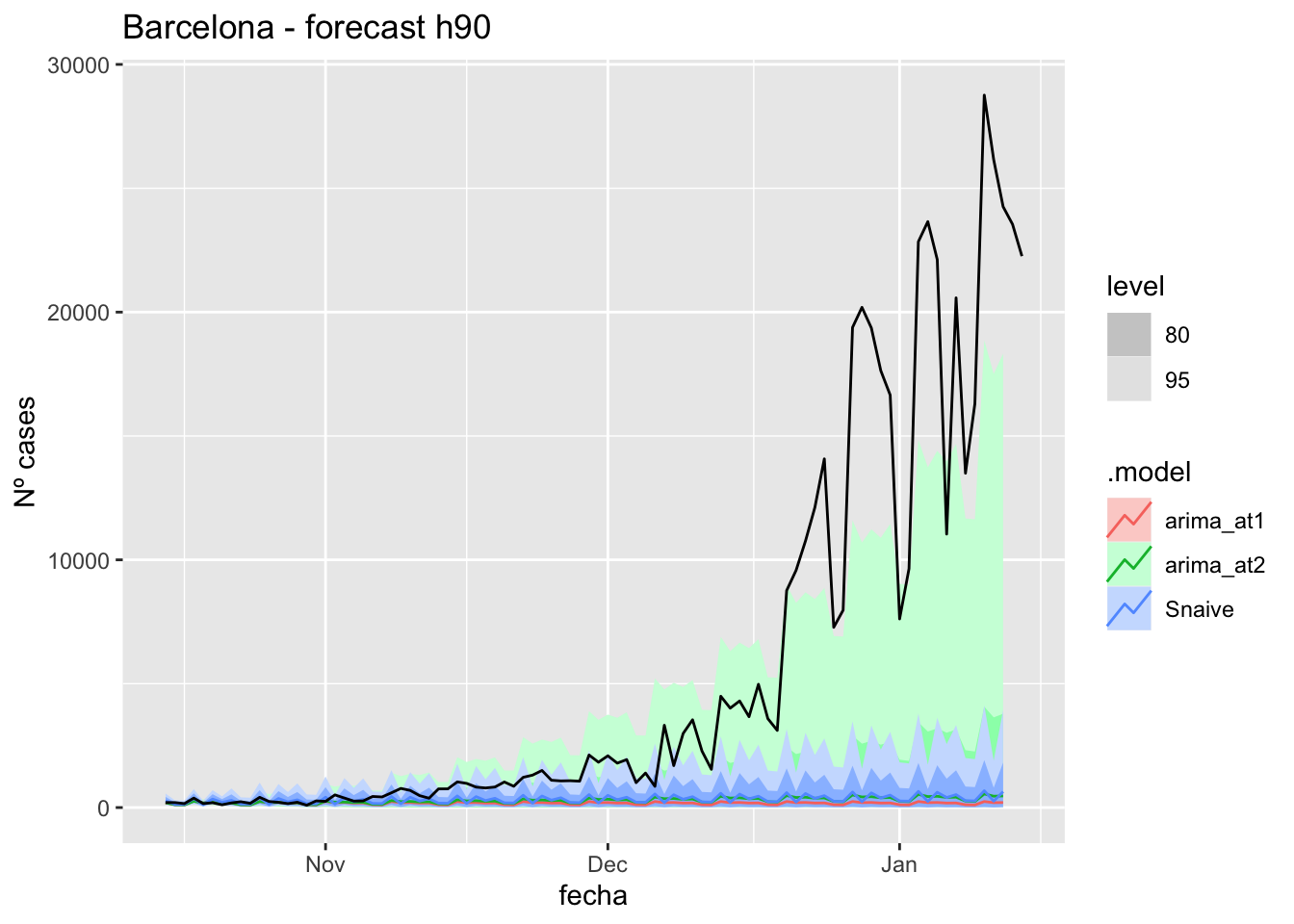
fc_h90 %>%
      autoplot(
            data_barcelona %>%
                  filter(fecha <= as.Date("2021-10-14", format = "%Y-%m-%d")+days(92) &
                               fecha > as.Date("2021-07-01", format = "%Y-%m-%d"))
      ) +
      labs(y = "Nº cases", title = "Barcelona - forecast h90")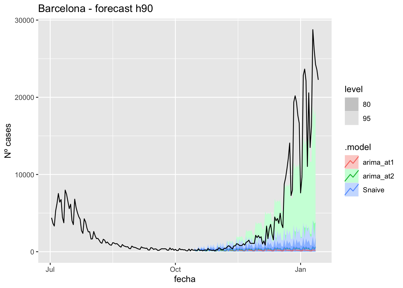
# Accuracy
fabletools::accuracy(fc_h90, data_barcelona)
# A tibble: 3 × 11
.model provincia .type ME RMSE MAE MPE MAPE MASE RMSSE ACF1
<chr> <chr> <chr> <dbl> <dbl> <dbl> <dbl> <dbl> <dbl> <dbl> <dbl>
1 arima_at1 Barcelona Test 5068. 9027. 5072. 71.8 74.8 13.5 13.6 0.868
2 arima_at2 Barcelona Test 4960. 8907. 4964. 67.8 70.8 13.2 13.4 0.868
3 Snaive Barcelona Test 4916. 8890. 4939. 58.7 71.4 13.1 13.4 0.870Madrid
data_madrid <- covid_data %>%
      filter(provincia == "Madrid") %>%
      filter(fecha > as.Date("2020-06-14", format = "%Y-%m-%d")) %>%
      select(provincia, fecha, num_casos, num_hosp, tmed,mob_grocery_pharmacy, mob_parks,
             mob_residential, mob_retail_recreation, mob_transit_stations, mob_workplaces, mob_flujo) %>%
      drop_na(-mob_flujo) %>%
      as_tsibble(key = provincia, index = fecha)
data_madrid
# A tsibble: 653 x 12 [1D]
# Key: provincia [1]
provincia fecha num_casos num_hosp tmed mob_grocery_pharmacy mob_parks
<chr> <date> <dbl> <dbl> <dbl> <dbl> <dbl>
1 Madrid 2020-06-15 153 10 20.7 -8 34
2 Madrid 2020-06-16 91 16 21 -8 21
3 Madrid 2020-06-17 93 14 20.2 -5 34
4 Madrid 2020-06-18 85 17 21.9 -7 30
5 Madrid 2020-06-19 78 20 22.6 -9 22
6 Madrid 2020-06-20 67 20 23.4 -12 25
7 Madrid 2020-06-21 42 3 25 -13 14
8 Madrid 2020-06-22 60 16 27.3 -8 29
9 Madrid 2020-06-23 68 11 28.4 -9 23
10 Madrid 2020-06-24 49 15 28 -7 22
# … with 643 more rows, and 5 more variables: mob_residential <dbl>,
# mob_retail_recreation <dbl>, mob_transit_stations <dbl>,
# mob_workplaces <dbl>, mob_flujo <dbl>data_madrid_train <- data_madrid %>%
filter(fecha <= as.Date("2021-10-14", format = "%Y-%m-%d"))
summary(data_madrid_train$fecha) Min. 1st Qu. Median Mean 3rd Qu. Max.
"2020-06-15" "2020-10-14" "2021-02-13" "2021-02-13" "2021-06-14" "2021-10-14" data_madrid_test <- data_madrid %>%
filter(fecha > as.Date("2021-10-14", format = "%Y-%m-%d"))
summary(data_madrid_test$fecha) Min. 1st Qu. Median Mean 3rd Qu. Max.
"2021-10-15" "2021-11-25" "2022-01-05" "2022-01-05" "2022-02-15" "2022-03-29" lambda_Madrid <- data_madrid %>%
features(num_casos, features = guerrero) %>%
pull(lambda_guerrero)
fit_model <- data_madrid_train %>%
model(
arima_at1 = ARIMA(box_cox(num_casos, lambda_Madrid)),
arima_at2 = ARIMA(box_cox(num_casos, lambda_Madrid),
stepwise = FALSE, approx = FALSE),
Snaive = SNAIVE(box_cox(num_casos, lambda_Madrid))
)
# Show and report model
fit_model# A mable: 1 x 4
# Key: provincia [1]
provincia arima_at1 arima_at2 Snaive
<chr> <model> <model> <model>
1 Madrid <ARIMA(2,1,1)(1,1,1)[7]> <ARIMA(2,1,1)(1,1,1)[7]> <SNAIVE>glance(fit_model)# A tibble: 3 × 9
provincia .model sigma2 log_lik AIC AICc BIC ar_roots ma_roots
<chr> <chr> <dbl> <dbl> <dbl> <dbl> <dbl> <list> <list>
1 Madrid arima_at1 0.0667 -33.4 78.8 79.0 104. <cpl [9]> <cpl [8]>
2 Madrid arima_at2 0.0667 -33.4 78.8 79.0 104. <cpl [9]> <cpl [8]>
3 Madrid Snaive 0.291 NA NA NA NA <NULL> <NULL> fit_model %>%
pivot_longer(-provincia,
names_to = ".model",
values_to = "orders") %>%
left_join(glance(fit_model), by = c("provincia", ".model")) %>%
arrange(AICc) %>%
select(.model:BIC)# A mable: 3 x 7
# Key: .model [3]
.model orders sigma2 log_lik AIC AICc BIC
<chr> <model> <dbl> <dbl> <dbl> <dbl> <dbl>
1 arima_at1 <ARIMA(2,1,1)(1,1,1)[7]> 0.0667 -33.4 78.8 79.0 104.
2 arima_at2 <ARIMA(2,1,1)(1,1,1)[7]> 0.0667 -33.4 78.8 79.0 104.
3 Snaive <SNAIVE> 0.291 NA NA NA NA # We use a Ljung-Box test >> large p-value, confirms residuals are similar / considered to white noise
fit_model %>%
select(Snaive) %>%
gg_tsresiduals()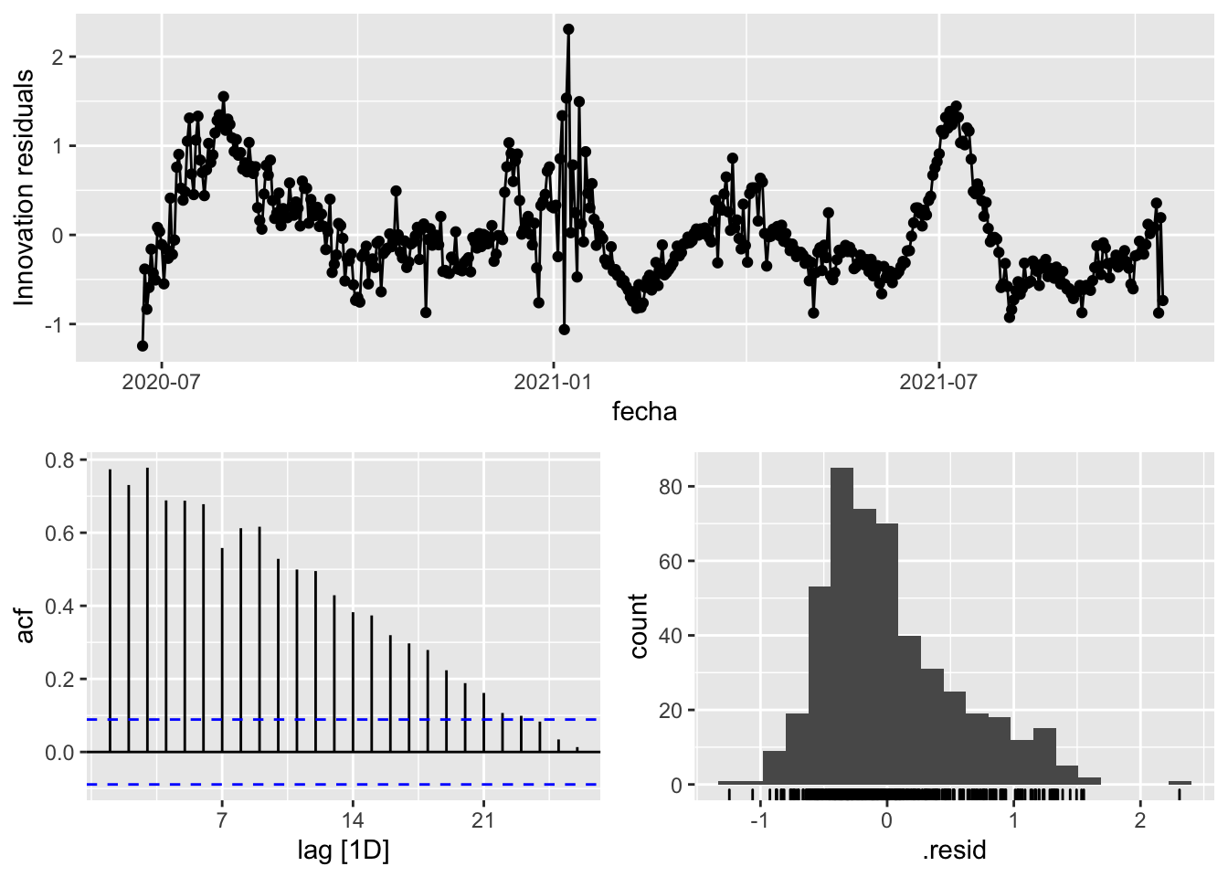
fit_model %>%
      select(arima_at1) %>%
      gg_tsresiduals()
fit_model %>%
      select(arima_at2) %>%
      gg_tsresiduals()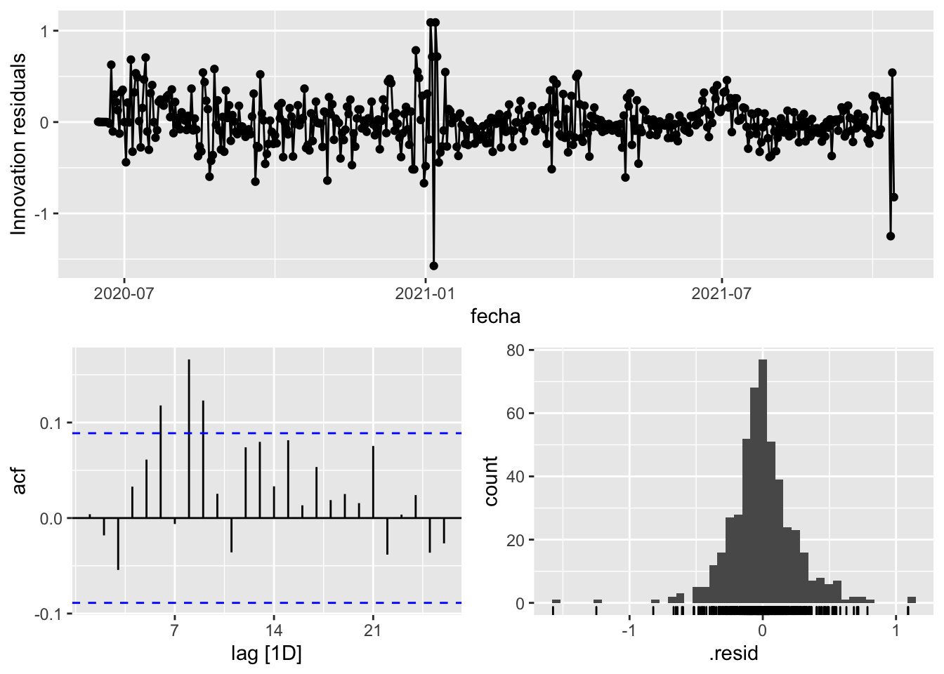
augment(fit_model) %>%
      features(.innov, ljung_box, lag=7)
# A tibble: 3 × 4
provincia .model lb_stat lb_pvalue
<chr> <chr> <dbl> <dbl>
1 Madrid arima_at1 10.9 0.143
2 Madrid arima_at2 10.9 0.143
3 Madrid Snaive 1678. 0 augment(fit_model) %>%
features(.innov, ljung_box, lag=14)# A tibble: 3 × 4
provincia .model lb_stat lb_pvalue
<chr> <chr> <dbl> <dbl>
1 Madrid arima_at1 39.6 0.000292
2 Madrid arima_at2 39.6 0.000292
3 Madrid Snaive 2594. 0 augment(fit_model) %>%
features(.innov, ljung_box, lag=21)# A tibble: 3 × 4
provincia .model lb_stat lb_pvalue
<chr> <chr> <dbl> <dbl>
1 Madrid arima_at1 48.0 0.000679
2 Madrid arima_at2 48.0 0.000679
3 Madrid Snaive 2854. 0 augment(fit_model) %>%
features(.innov, ljung_box, lag=90)# A tibble: 3 × 4
provincia .model lb_stat lb_pvalue
<chr> <chr> <dbl> <dbl>
1 Madrid arima_at1 105. 0.130
2 Madrid arima_at2 105. 0.130
3 Madrid Snaive 3856. 0 # Significant spikes out of 30 is still consistent with white noise
# To be sure, use a Ljung-Box test, which has a large p-value, confirming that
# the residuals are similar to white noise.
# Note that the alternative models also passed this test.
#
# Forecast
fc_h7 <- fabletools::forecast(fit_model, h = 7)
fc_h14 <- fabletools::forecast(fit_model, h = 14)
fc_h21 <- fabletools::forecast(fit_model, h = 21)
fc_h90 <- fabletools::forecast(fit_model, h = 90)7 days
# Plots
fc_h7 %>%
      autoplot(
            data_madrid_test %>%
                  filter(fecha <= as.Date("2021-10-14", format = "%Y-%m-%d")+days(9))
      ) +
      labs(y = "Nº cases", title = "Madrid - forecast h7")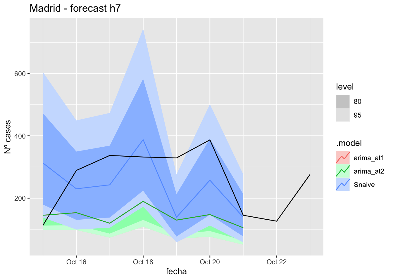
fc_h7 %>%
      autoplot(
            data_madrid %>%
                  filter(fecha <= as.Date("2021-10-14", format = "%Y-%m-%d")+days(9) &
                               fecha > as.Date("2021-07-01", format = "%Y-%m-%d"))
      ) +
      labs(y = "Nº cases", title = "Madrid - forecast h7")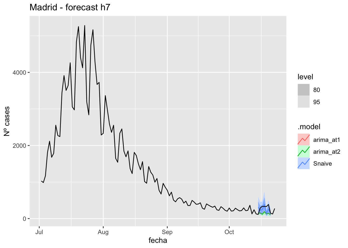
# Accuracy
fabletools::accuracy(fc_h7, data_madrid)
# A tibble: 3 × 11
.model provincia .type ME RMSE MAE MPE MAPE MASE RMSSE ACF1
<chr> <chr> <chr> <dbl> <dbl> <dbl> <dbl> <dbl> <dbl> <dbl> <dbl>
1 arima_at1 Madrid Test 135. 163. 144. 39.5 47.6 0.339 0.243 -0.0355
2 arima_at2 Madrid Test 135. 163. 144. 39.5 47.6 0.339 0.243 -0.0355
3 Snaive Madrid Test 32.1 124. 105. -7.03 48.2 0.247 0.185 -0.109 14 days
# Plots
fc_h14 %>%
      autoplot(
            data_madrid_test %>%
                  filter(fecha <= as.Date("2021-10-14", format = "%Y-%m-%d")+days(16))
      ) +
      labs(y = "Nº cases", title = "Madrid - forecast h14")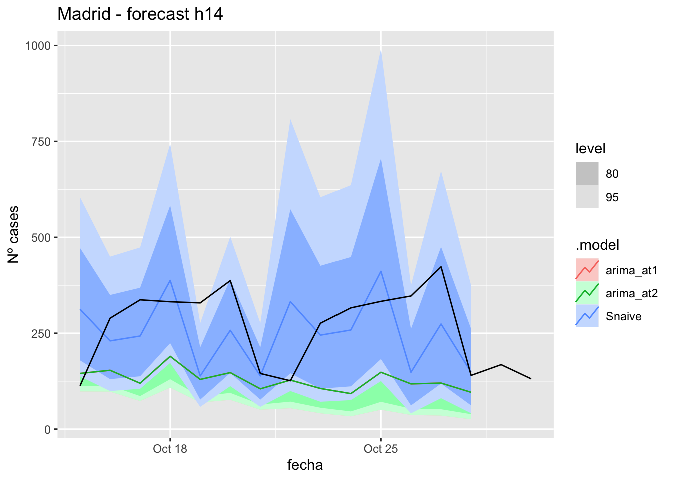
fc_h14 %>%
      autoplot(
            data_madrid %>%
                  filter(fecha <= as.Date("2021-10-14", format = "%Y-%m-%d")+days(16) &
                               fecha > as.Date("2021-07-01", format = "%Y-%m-%d"))
      ) +
      labs(y = "Nº cases", title = "Madrid - forecast h14")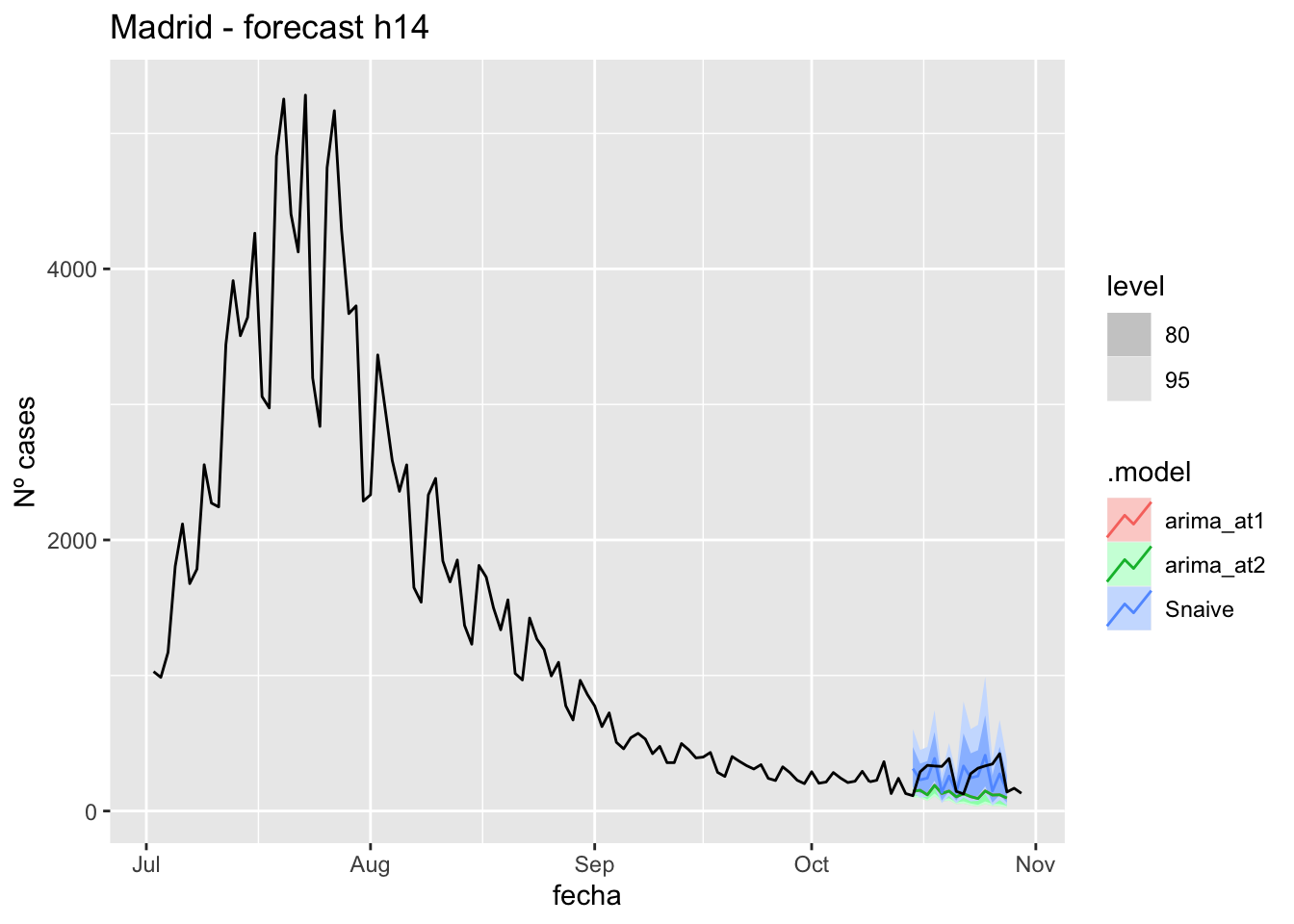
# Accuracy
fabletools::accuracy(fc_h14, data_madrid)
# A tibble: 3 × 11
.model provincia .type ME RMSE MAE MPE MAPE MASE RMSSE ACF1
<chr> <chr> <chr> <dbl> <dbl> <dbl> <dbl> <dbl> <dbl> <dbl> <dbl>
1 arima_at1 Madrid Test 150. 178. 155. 45.1 49.4 0.364 0.265 0.0892
2 arima_at2 Madrid Test 150. 178. 155. 45.1 49.4 0.364 0.265 0.0892
3 Snaive Madrid Test 26.3 126. 105. -8.58 46.6 0.246 0.188 -0.047221 days
# Plots
fc_h21 %>%
      autoplot(
            data_madrid_test %>%
                  filter(fecha <= as.Date("2021-10-14", format = "%Y-%m-%d")+days(23))
      ) +
      labs(y = "Nº cases", title = "Madrid - forecast h21")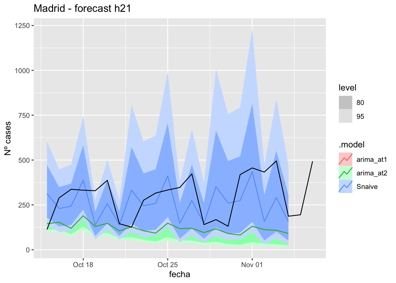
fc_h21 %>%
      autoplot(
            data_madrid %>%
                  filter(fecha <= as.Date("2021-10-14", format = "%Y-%m-%d")+days(23) &
                               fecha > as.Date("2021-07-01", format = "%Y-%m-%d"))
      ) +
      labs(y = "Nº cases", title = "Madrid - forecast h21")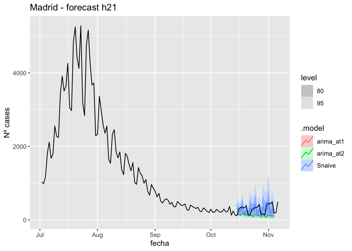
# Accuracy
fabletools::accuracy(fc_h21, data_madrid)
# A tibble: 3 × 11
.model provincia .type ME RMSE MAE MPE MAPE MASE RMSSE ACF1
<chr> <chr> <chr> <dbl> <dbl> <dbl> <dbl> <dbl> <dbl> <dbl> <dbl>
1 arima_at1 Madrid Test 174. 210. 177. 50.0 52.8 0.418 0.313 0.287
2 arima_at2 Madrid Test 174. 210. 177. 50.0 52.8 0.418 0.313 0.287
3 Snaive Madrid Test 34.8 140. 117. -8.01 48.6 0.275 0.209 0.13190 days
# Plots
fc_h90 %>%
      autoplot(
            data_madrid_test %>%
                  filter(fecha <= as.Date("2021-10-14", format = "%Y-%m-%d")+days(92))
      ) +
      labs(y = "Nº cases", title = "Madrid - forecast h90")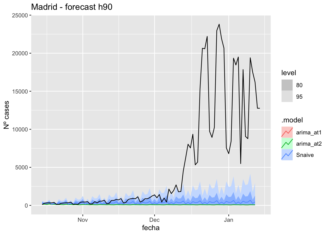
fc_h90 %>%
      autoplot(
            data_madrid %>%
                  filter(fecha <= as.Date("2021-10-14", format = "%Y-%m-%d")+days(92) &
                               fecha > as.Date("2021-07-01", format = "%Y-%m-%d"))
      ) +
      labs(y = "Nº cases", title = "Madrid - forecast h90")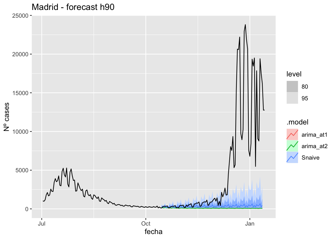
# Accuracy
fabletools::accuracy(fc_h90, data_madrid)
# A tibble: 3 × 11
.model provincia .type ME RMSE MAE MPE MAPE MASE RMSSE ACF1
<chr> <chr> <chr> <dbl> <dbl> <dbl> <dbl> <dbl> <dbl> <dbl> <dbl>
1 arima_at1 Madrid Test 5007. 8744. 5008. 81.7 82.4 11.8 13.0 0.840
2 arima_at2 Madrid Test 5007. 8744. 5008. 81.7 82.4 11.8 13.0 0.840
3 Snaive Madrid Test 4763. 8564. 4792. 51.8 68.9 11.3 12.7 0.840Málaga
data_malaga <- covid_data %>%
      filter(provincia == "Málaga") %>%
      filter(fecha > as.Date("2020-06-14", format = "%Y-%m-%d")) %>%
      select(provincia, fecha, num_casos, num_hosp, tmed,mob_grocery_pharmacy, mob_parks,
             mob_residential, mob_retail_recreation, mob_transit_stations, mob_workplaces, mob_flujo) %>%
      drop_na(-mob_flujo) %>%
      as_tsibble(key = provincia, index = fecha)
data_malaga
# A tsibble: 653 x 12 [1D]
# Key: provincia [1]
provincia fecha num_casos num_hosp tmed mob_grocery_pharmacy mob_parks
<chr> <date> <dbl> <dbl> <dbl> <dbl> <dbl>
1 Málaga 2020-06-15 1 0 27.2 -16 -9
2 Málaga 2020-06-16 1 0 27.8 -13 -4
3 Málaga 2020-06-17 2 0 26.9 -13 1
4 Málaga 2020-06-18 2 1 21.6 -12 3
5 Málaga 2020-06-19 1 0 24.7 -12 2
6 Málaga 2020-06-20 4 0 22.6 -14 8
7 Málaga 2020-06-21 4 0 22.7 -16 -3
8 Málaga 2020-06-22 6 0 25 -13 1
9 Málaga 2020-06-23 8 0 25.6 -10 18
10 Málaga 2020-06-24 65 2 24.5 -13 12
# … with 643 more rows, and 5 more variables: mob_residential <dbl>,
# mob_retail_recreation <dbl>, mob_transit_stations <dbl>,
# mob_workplaces <dbl>, mob_flujo <dbl>data_malaga_train <- data_malaga %>%
filter(fecha <= as.Date("2021-10-14", format = "%Y-%m-%d"))
summary(data_malaga_train$fecha) Min. 1st Qu. Median Mean 3rd Qu. Max.
"2020-06-15" "2020-10-14" "2021-02-13" "2021-02-13" "2021-06-14" "2021-10-14" data_malaga_test <- data_malaga %>%
filter(fecha > as.Date("2021-10-14", format = "%Y-%m-%d"))
summary(data_malaga_test$fecha) Min. 1st Qu. Median Mean 3rd Qu. Max.
"2021-10-15" "2021-11-25" "2022-01-05" "2022-01-05" "2022-02-15" "2022-03-29" lambda_Malaga <- data_malaga %>%
features(num_casos, features = guerrero) %>%
pull(lambda_guerrero)
fit_model <- data_malaga_train %>%
model(
arima_at1 = ARIMA(box_cox(num_casos, lambda_Malaga)),
arima_at2 = ARIMA(box_cox(num_casos, lambda_Malaga),
stepwise = FALSE, approx = FALSE),
Snaive = SNAIVE(box_cox(num_casos, lambda_Malaga))
)
# Show and report model
fit_model# A mable: 1 x 4
# Key: provincia [1]
provincia arima_at1 arima_at2 Snaive
<chr> <model> <model> <model>
1 Málaga <ARIMA(4,1,0)(1,1,1)[7]> <ARIMA(1,1,3)(0,1,1)[7]> <SNAIVE>glance(fit_model)# A tibble: 3 × 9
provincia .model sigma2 log_lik AIC AICc BIC ar_roots ma_roots
<chr> <chr> <dbl> <dbl> <dbl> <dbl> <dbl> <list> <list>
1 Málaga arima_at1 0.518 -525. 1063. 1064. 1093. <cpl [11]> <cpl [7]>
2 Málaga arima_at2 0.504 -518. 1049. 1049. 1074. <cpl [1]> <cpl [10]>
3 Málaga Snaive 2.15 NA NA NA NA <NULL> <NULL> fit_model %>%
pivot_longer(-provincia,
names_to = ".model",
values_to = "orders") %>%
left_join(glance(fit_model), by = c("provincia", ".model")) %>%
arrange(AICc) %>%
select(.model:BIC)# A mable: 3 x 7
# Key: .model [3]
.model orders sigma2 log_lik AIC AICc BIC
<chr> <model> <dbl> <dbl> <dbl> <dbl> <dbl>
1 arima_at2 <ARIMA(1,1,3)(0,1,1)[7]> 0.504 -518. 1049. 1049. 1074.
2 arima_at1 <ARIMA(4,1,0)(1,1,1)[7]> 0.518 -525. 1063. 1064. 1093.
3 Snaive <SNAIVE> 2.15 NA NA NA NA # We use a Ljung-Box test >> large p-value, confirms residuals are similar / considered to white noise
fit_model %>%
select(Snaive) %>%
gg_tsresiduals()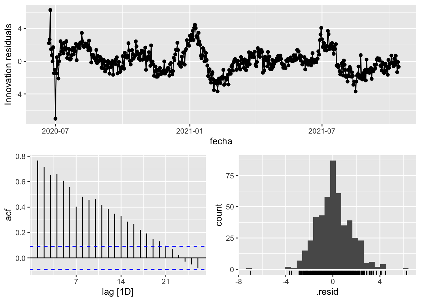
fit_model %>%
      select(arima_at1) %>%
      gg_tsresiduals()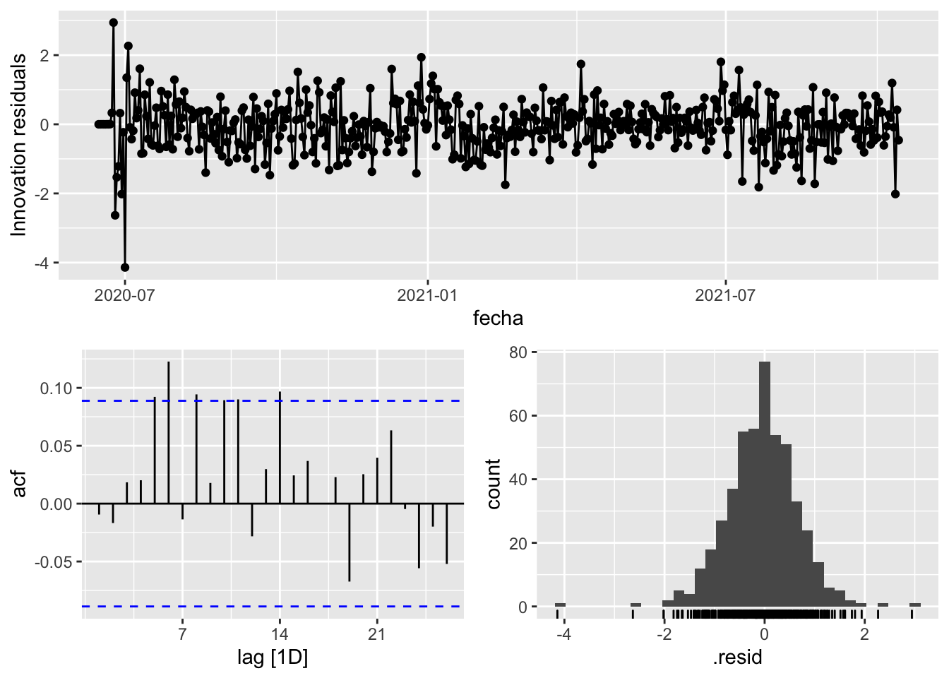
fit_model %>%
      select(arima_at2) %>%
      gg_tsresiduals()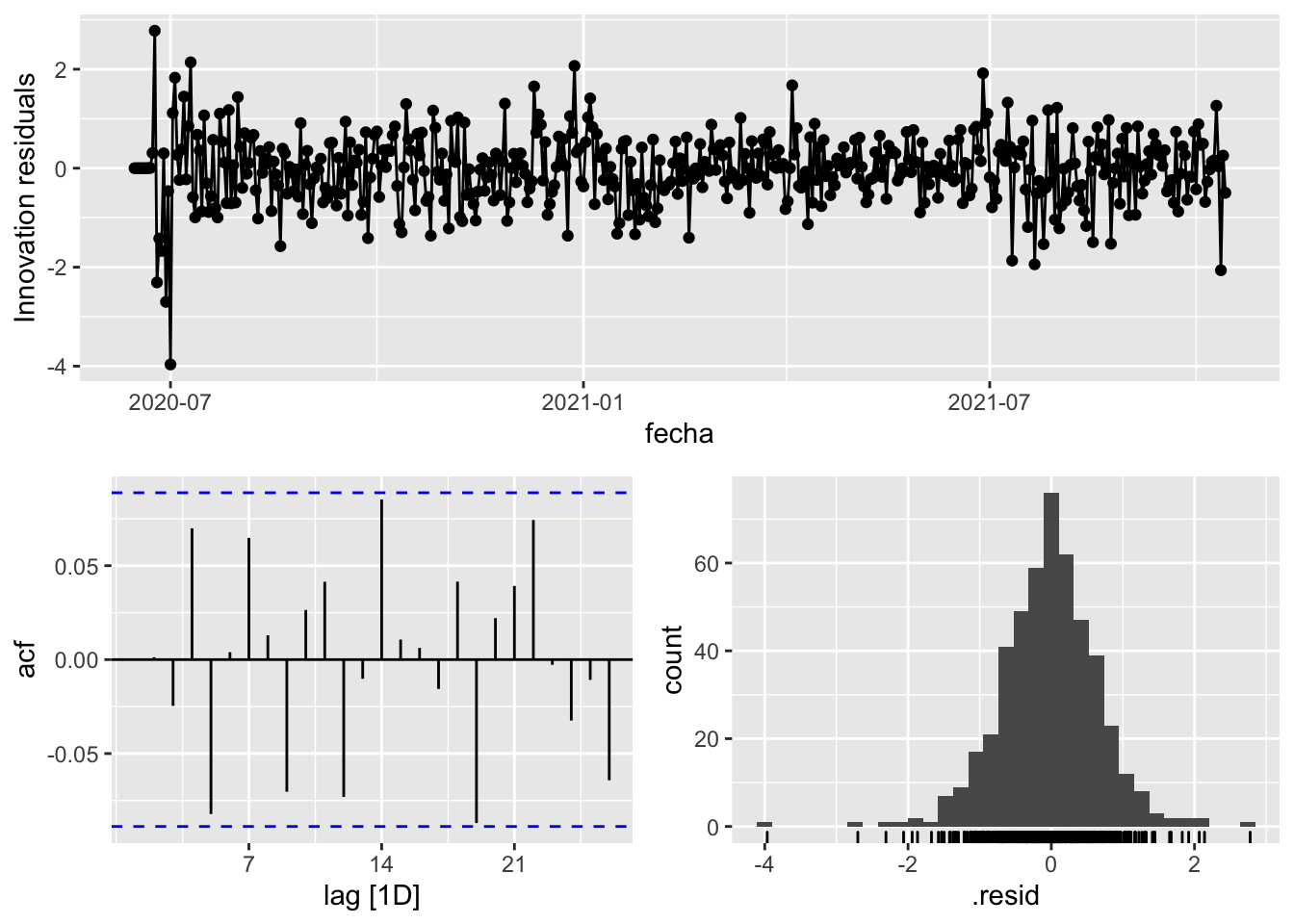
augment(fit_model) %>%
      features(.innov, ljung_box, lag=7)
# A tibble: 3 × 4
provincia .model lb_stat lb_pvalue
<chr> <chr> <dbl> <dbl>
1 Málaga arima_at1 12.3 0.0912
2 Málaga arima_at2 8.13 0.321
3 Málaga Snaive 1361. 0 augment(fit_model) %>%
features(.innov, ljung_box, lag=14)# A tibble: 3 × 4
provincia .model lb_stat lb_pvalue
<chr> <chr> <dbl> <dbl>
1 Málaga arima_at1 30.5 0.00654
2 Málaga arima_at2 18.3 0.195
3 Málaga Snaive 1956. 0 augment(fit_model) %>%
features(.innov, ljung_box, lag=21)# A tibble: 3 × 4
provincia .model lb_stat lb_pvalue
<chr> <chr> <dbl> <dbl>
1 Málaga arima_at1 35.2 0.0270
2 Málaga arima_at2 24.2 0.282
3 Málaga Snaive 2100. 0 augment(fit_model) %>%
features(.innov, ljung_box, lag=90)# A tibble: 3 × 4
provincia .model lb_stat lb_pvalue
<chr> <chr> <dbl> <dbl>
1 Málaga arima_at1 130. 0.00387
2 Málaga arima_at2 85.1 0.627
3 Málaga Snaive 3195. 0 # Significant spikes out of 30 is still consistent with white noise
# To be sure, use a Ljung-Box test, which has a large p-value, confirming that
# the residuals are similar to white noise.
# Note that the alternative models also passed this test.
#
# Forecast
fc_h7 <- fabletools::forecast(fit_model, h = 7)
fc_h14 <- fabletools::forecast(fit_model, h = 14)
fc_h21 <- fabletools::forecast(fit_model, h = 21)
fc_h90 <- fabletools::forecast(fit_model, h = 90)7 days
# Plots
fc_h7 %>%
      autoplot(
            data_malaga_test %>%
                  filter(fecha <= as.Date("2021-10-14", format = "%Y-%m-%d")+days(9))
      ) +
      labs(y = "Nº cases", title = "Malaga - forecast h7")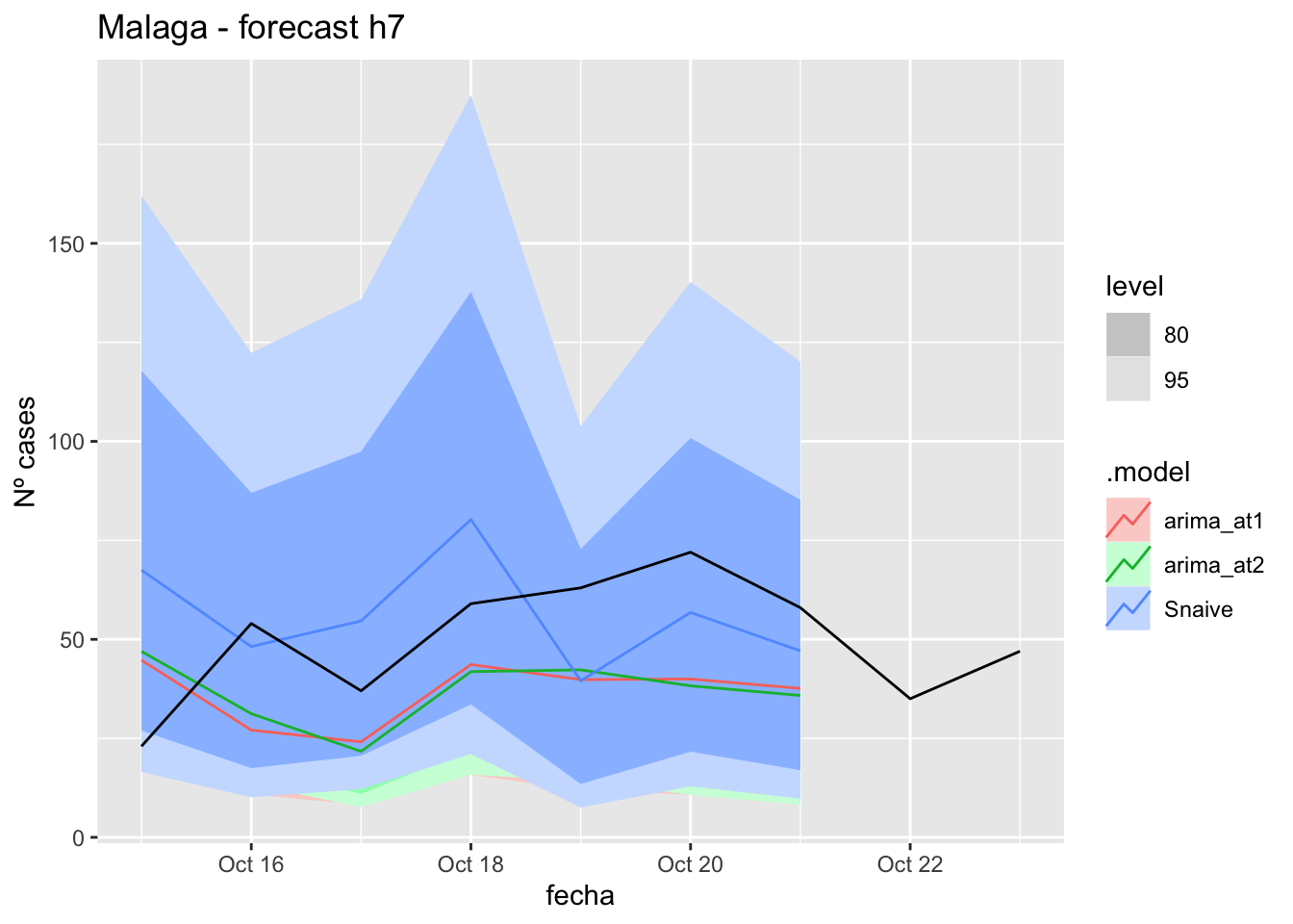
fc_h7 %>%
      autoplot(
            data_malaga %>%
                  filter(fecha <= as.Date("2021-10-14", format = "%Y-%m-%d")+days(9) &
                               fecha > as.Date("2021-07-01", format = "%Y-%m-%d"))
      ) +
      labs(y = "Nº cases", title = "Malaga - forecast h7")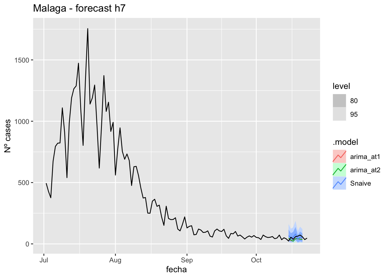
# Accuracy
fabletools::accuracy(fc_h7, data_malaga)
# A tibble: 3 × 11
.model provincia .type ME RMSE MAE MPE MAPE MASE RMSSE ACF1
<chr> <chr> <chr> <dbl> <dbl> <dbl> <dbl> <dbl> <dbl> <dbl> <dbl>
1 arima_at1 Málaga Test 15.6 22.6 21.8 18.9 46.0 0.221 0.134 -0.133
2 arima_at2 Málaga Test 15.4 22.9 22.3 18.1 47.8 0.226 0.135 -0.0302
3 Snaive Málaga Test -4.00 22.9 19.8 -27.0 52.2 0.201 0.135 0.012314 days
# Plots
fc_h14 %>%
      autoplot(
            data_malaga_test %>%
                  filter(fecha <= as.Date("2021-10-14", format = "%Y-%m-%d")+days(16))
      ) +
      labs(y = "Nº cases", title = "Malaga - forecast h14")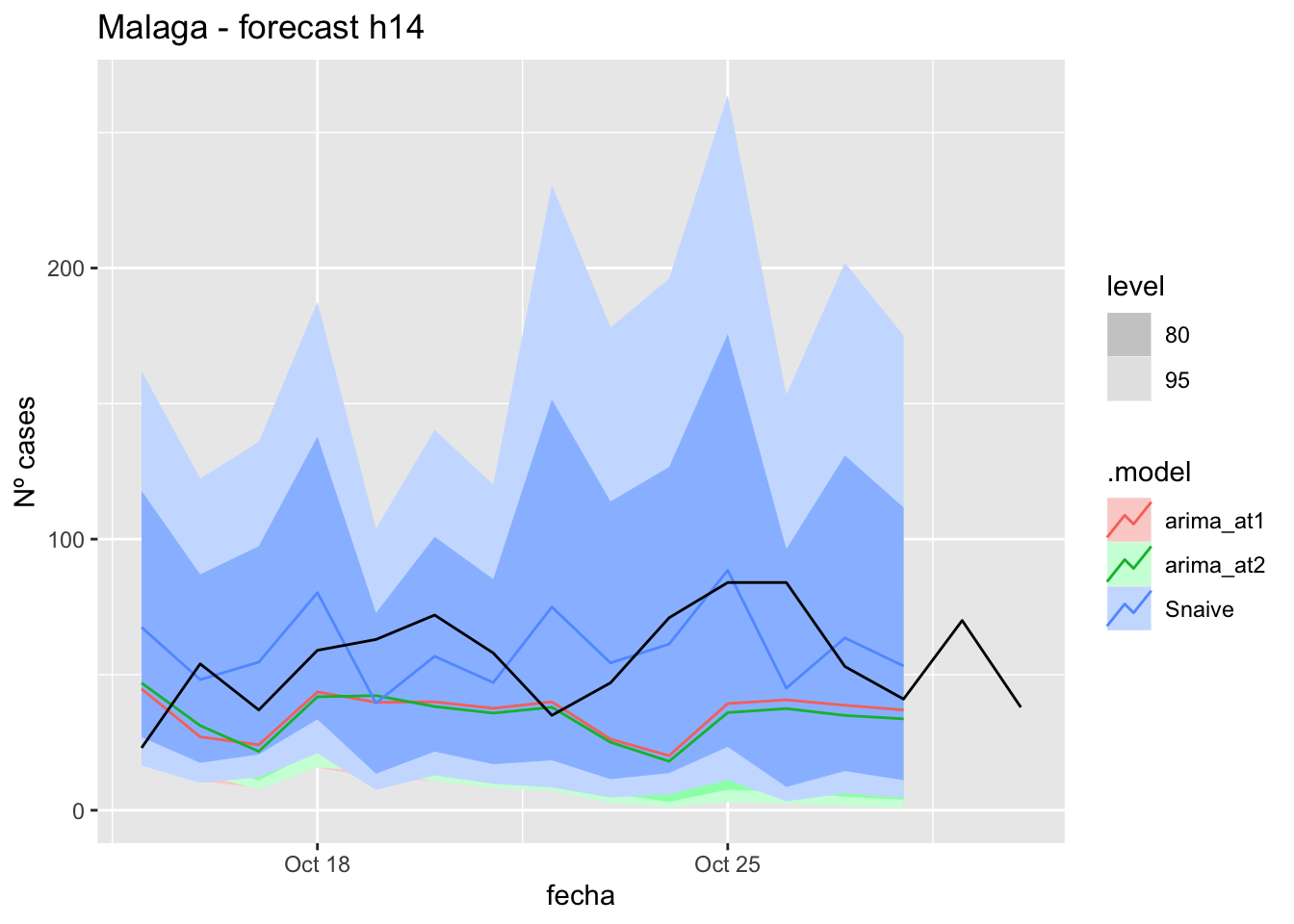
fc_h14 %>%
      autoplot(
            data_malaga %>%
                  filter(fecha <= as.Date("2021-10-14", format = "%Y-%m-%d")+days(16) &
                               fecha > as.Date("2021-07-01", format = "%Y-%m-%d"))
      ) +
      labs(y = "Nº cases", title = "Malaga - forecast h14")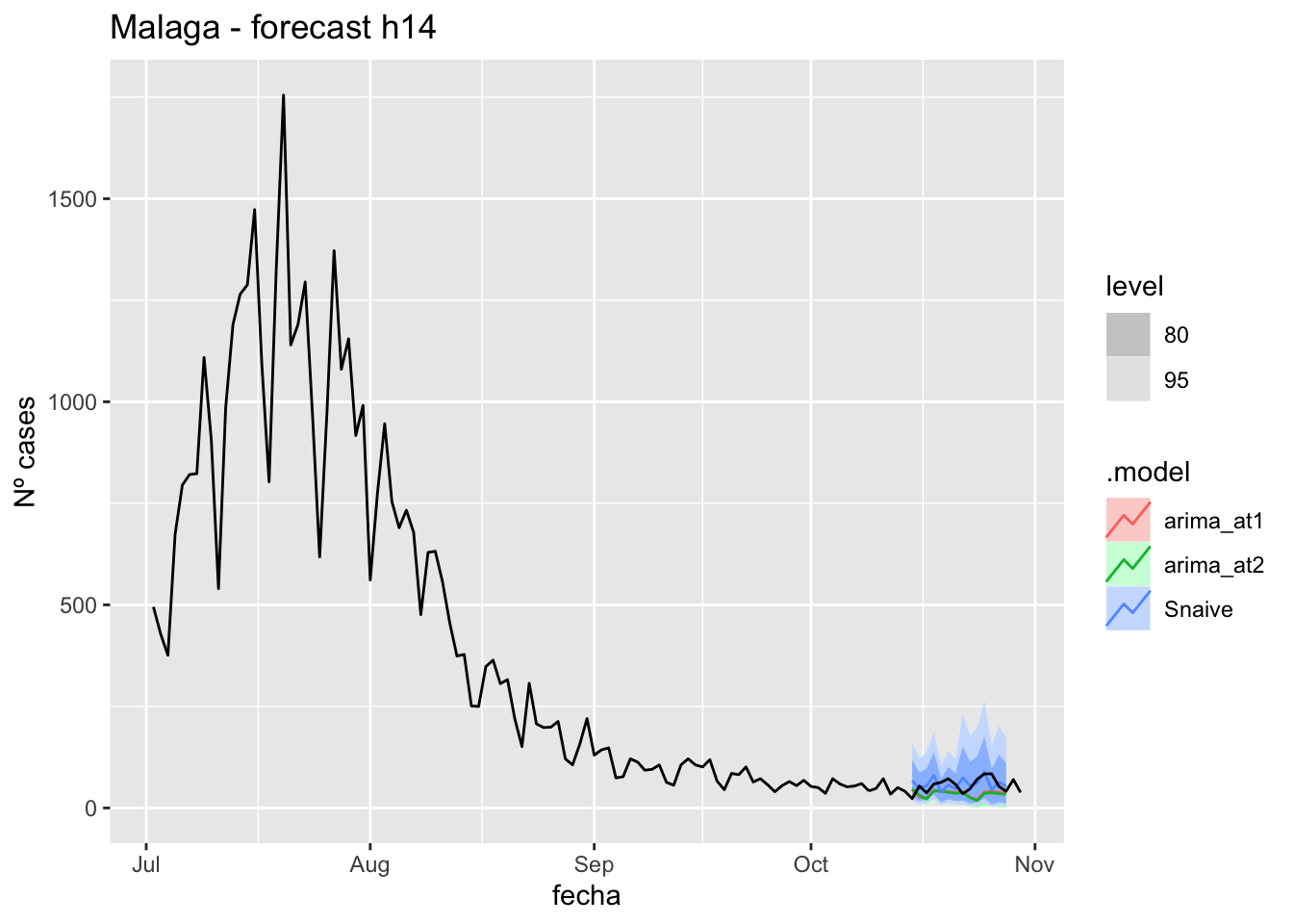
# Accuracy
fabletools::accuracy(fc_h14, data_malaga)
# A tibble: 3 × 11
.model provincia .type ME RMSE MAE MPE MAPE MASE RMSSE ACF1
<chr> <chr> <chr> <dbl> <dbl> <dbl> <dbl> <dbl> <dbl> <dbl> <dbl>
1 arima_at1 Málaga Test 20.1 27.7 24.0 26.8 42.4 0.243 0.163 0.199
2 arima_at2 Málaga Test 21.4 29.0 25.2 28.8 44.9 0.256 0.172 0.261
3 Snaive Málaga Test -3.86 22.7 18.7 -22.4 43.6 0.190 0.134 -0.097321 days
# Plots
fc_h21 %>%
      autoplot(
            data_malaga_test %>%
                  filter(fecha <= as.Date("2021-10-14", format = "%Y-%m-%d")+days(23))
      ) +
      labs(y = "Nº cases", title = "Malaga - forecast h21")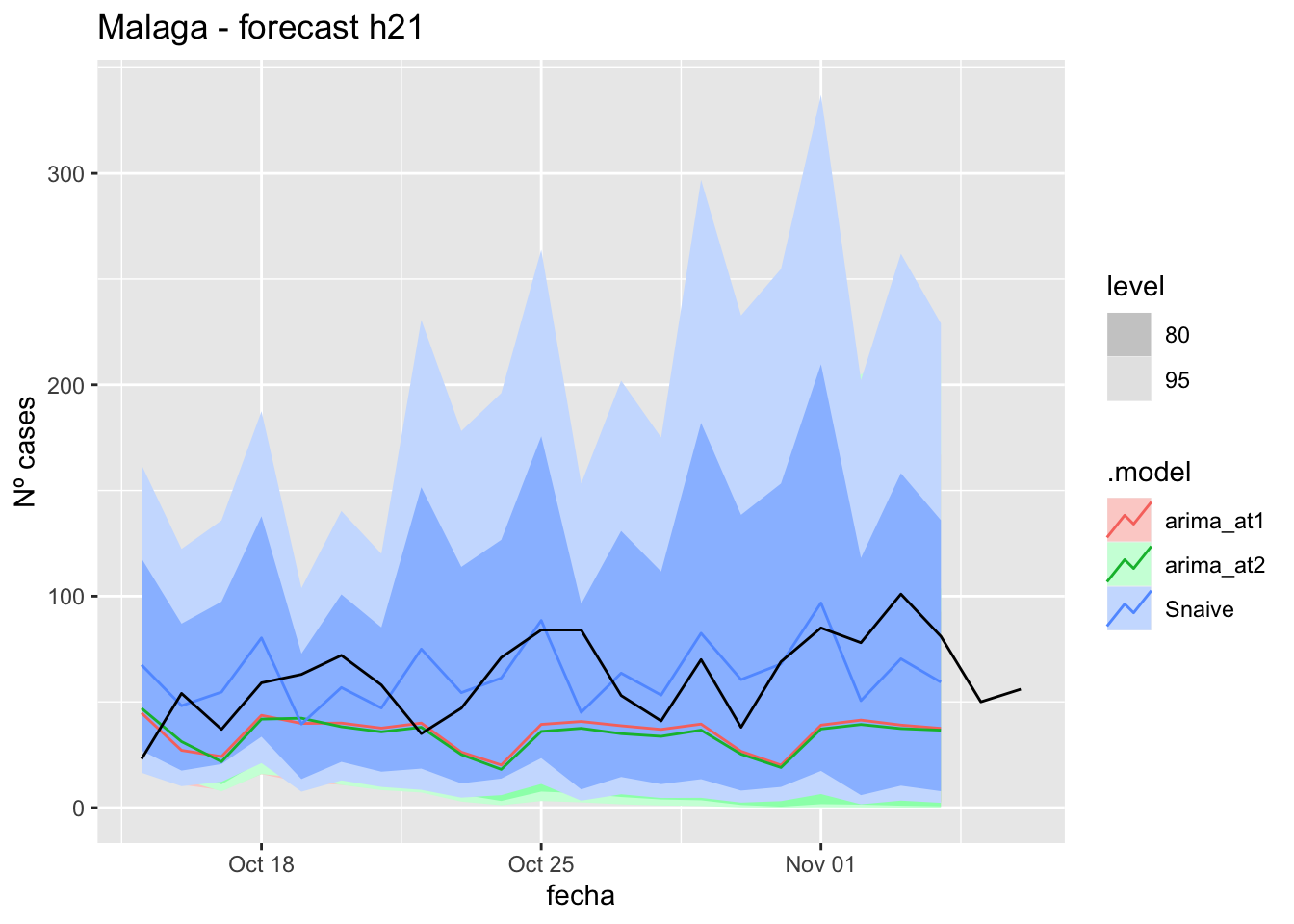
fc_h21 %>%
      autoplot(
            data_malaga %>%
                  filter(fecha <= as.Date("2021-10-14", format = "%Y-%m-%d")+days(23) &
                               fecha > as.Date("2021-07-01", format = "%Y-%m-%d"))
      ) +
      labs(y = "Nº cases", title = "Malaga - forecast h21")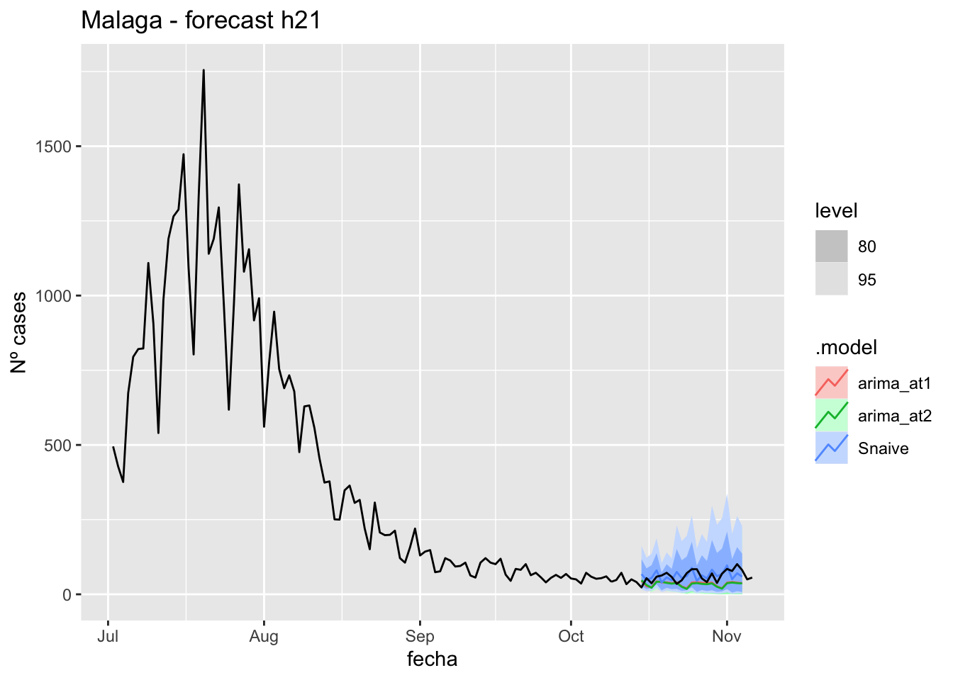
# Accuracy
fabletools::accuracy(fc_h21, data_malaga)
# A tibble: 3 × 11
.model provincia .type ME RMSE MAE MPE MAPE MASE RMSSE ACF1
<chr> <chr> <chr> <dbl> <dbl> <dbl> <dbl> <dbl> <dbl> <dbl> <dbl>
1 arima_at1 Málaga Test 26.7 33.3 29.2 35.0 45.4 0.297 0.197 0.270
2 arima_at2 Málaga Test 28.1 34.8 30.7 37.2 47.9 0.311 0.205 0.303
3 Snaive Málaga Test -0.951 22.0 18.6 -14.8 37.9 0.188 0.130 0.088690 days
# Plots
fc_h90 %>%
      autoplot(
            data_malaga_test %>%
                  filter(fecha <= as.Date("2021-10-14", format = "%Y-%m-%d")+days(92))
      ) +
      labs(y = "Nº cases", title = "Malaga - forecast h90")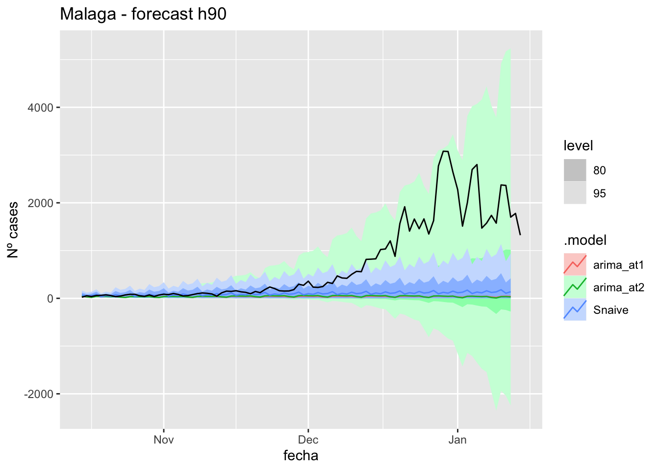
fc_h90 %>%
      autoplot(
            data_malaga %>%
                  filter(fecha <= as.Date("2021-10-14", format = "%Y-%m-%d")+days(92) &
                               fecha > as.Date("2021-07-01", format = "%Y-%m-%d"))
      ) +
      labs(y = "Nº cases", title = "Malaga - forecast h90")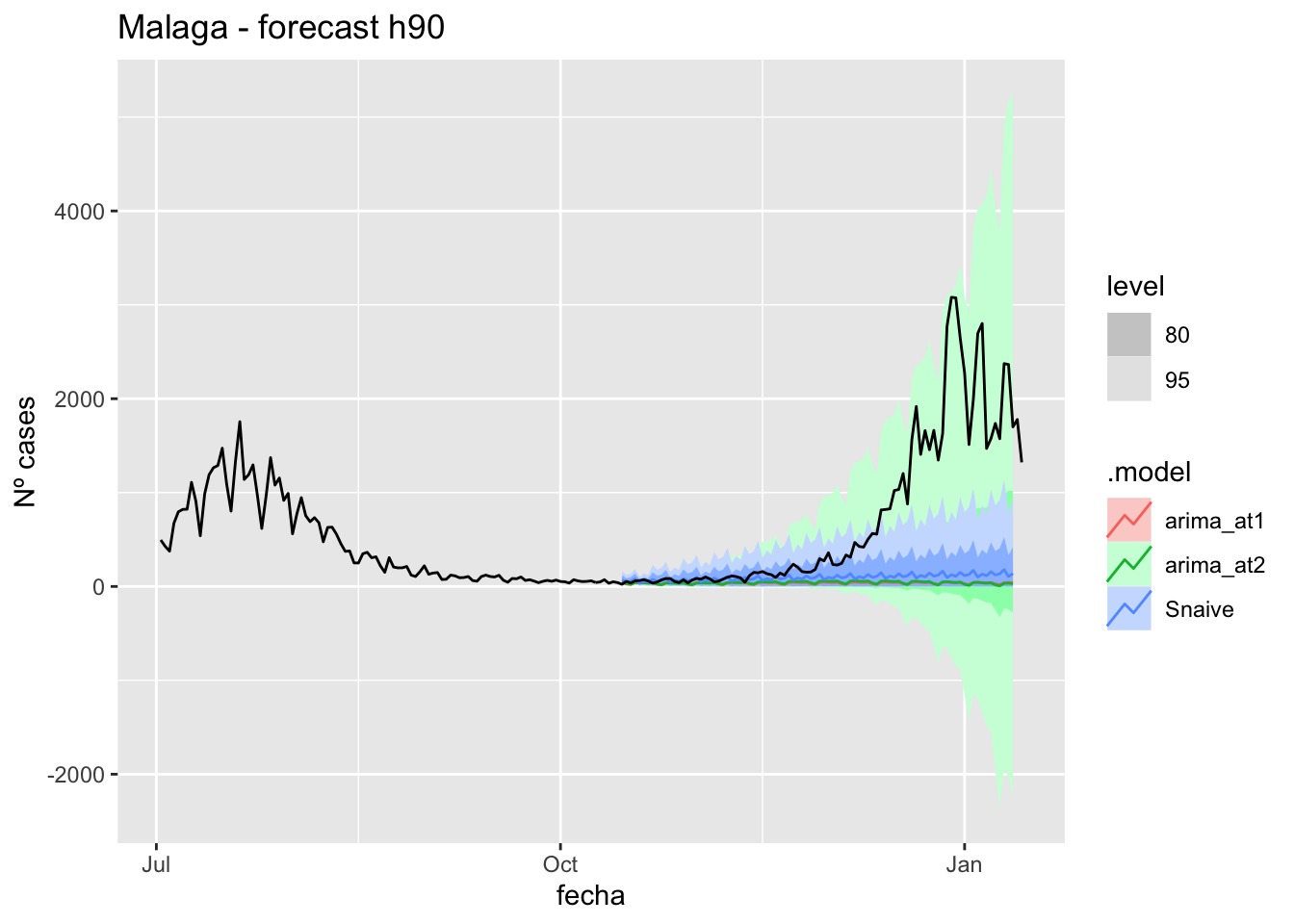
# Accuracy
fabletools::accuracy(fc_h90, data_malaga)
# A tibble: 3 × 11
.model provincia .type ME RMSE MAE MPE MAPE MASE RMSSE ACF1
<chr> <chr> <chr> <dbl> <dbl> <dbl> <dbl> <dbl> <dbl> <dbl> <dbl>
1 arima_at1 Málaga Test 680. 1100. 680. 73.4 75.9 6.91 6.50 0.934
2 arima_at2 Málaga Test 676. 1099. 677. 72.2 74.7 6.87 6.49 0.935
3 Snaive Málaga Test 620. 1049. 628. 44.9 62.3 6.37 6.20 0.929Sevilla
data_sevilla <- covid_data %>%
      filter(provincia == "Sevilla") %>%
      filter(fecha > as.Date("2020-06-14", format = "%Y-%m-%d")) %>%
      select(provincia, fecha, num_casos, num_hosp, tmed,mob_grocery_pharmacy, mob_parks,
             mob_residential, mob_retail_recreation, mob_transit_stations, mob_workplaces, mob_flujo) %>%
      drop_na(-mob_flujo) %>%
      as_tsibble(key = provincia, index = fecha)
data_sevilla
# A tsibble: 653 x 12 [1D]
# Key: provincia [1]
provincia fecha num_casos num_hosp tmed mob_grocery_pharmacy mob_parks
<chr> <date> <dbl> <dbl> <dbl> <dbl> <dbl>
1 Sevilla 2020-06-15 2 1 23.1 -14 -13
2 Sevilla 2020-06-16 1 0 24.0 -10 -4
3 Sevilla 2020-06-17 0 0 24.9 -10 -7
4 Sevilla 2020-06-18 0 0 25.8 -12 -13
5 Sevilla 2020-06-19 0 0 26.6 -13 -20
6 Sevilla 2020-06-20 0 0 27.5 -20 -34
7 Sevilla 2020-06-21 0 0 28.4 -27 -47
8 Sevilla 2020-06-22 1 0 29.3 -17 -19
9 Sevilla 2020-06-23 0 0 30.2 -12 -13
10 Sevilla 2020-06-24 1 0 29.4 -12 -12
# … with 643 more rows, and 5 more variables: mob_residential <dbl>,
# mob_retail_recreation <dbl>, mob_transit_stations <dbl>,
# mob_workplaces <dbl>, mob_flujo <dbl>data_sevilla_train <- data_sevilla %>%
filter(fecha <= as.Date("2021-10-14", format = "%Y-%m-%d"))
summary(data_sevilla_train$fecha) Min. 1st Qu. Median Mean 3rd Qu. Max.
"2020-06-15" "2020-10-14" "2021-02-13" "2021-02-13" "2021-06-14" "2021-10-14" data_sevilla_test <- data_sevilla %>%
filter(fecha > as.Date("2021-10-14", format = "%Y-%m-%d"))
summary(data_sevilla_test$fecha) Min. 1st Qu. Median Mean 3rd Qu. Max.
"2021-10-15" "2021-11-25" "2022-01-05" "2022-01-05" "2022-02-15" "2022-03-29" lambda_Sevilla <- data_sevilla %>%
features(num_casos, features = guerrero) %>%
pull(lambda_guerrero)
fit_model <- data_sevilla_train %>%
model(
arima_at1 = ARIMA(box_cox(num_casos, lambda_Sevilla)),
arima_at2 = ARIMA(box_cox(num_casos, lambda_Sevilla),
stepwise = FALSE, approx = FALSE),
Snaive = SNAIVE(box_cox(num_casos, lambda_Sevilla))
)
# Show and report model
fit_model# A mable: 1 x 4
# Key: provincia [1]
provincia arima_at1 arima_at2 Snaive
<chr> <model> <model> <model>
1 Sevilla <ARIMA(3,1,1)(2,0,0)[7]> <ARIMA(4,1,0)(2,0,0)[7]> <SNAIVE>glance(fit_model)# A tibble: 3 × 9
provincia .model sigma2 log_lik AIC AICc BIC ar_roots ma_roots
<chr> <chr> <dbl> <dbl> <dbl> <dbl> <dbl> <list> <list>
1 Sevilla arima_at1 0.924 -670. 1353. 1354. 1383. <cpl [17]> <cpl [1]>
2 Sevilla arima_at2 0.922 -669. 1353. 1353. 1382. <cpl [18]> <cpl [0]>
3 Sevilla Snaive 2.02 NA NA NA NA <NULL> <NULL> fit_model %>%
pivot_longer(-provincia,
names_to = ".model",
values_to = "orders") %>%
left_join(glance(fit_model), by = c("provincia", ".model")) %>%
arrange(AICc) %>%
select(.model:BIC)# A mable: 3 x 7
# Key: .model [3]
.model orders sigma2 log_lik AIC AICc BIC
<chr> <model> <dbl> <dbl> <dbl> <dbl> <dbl>
1 arima_at2 <ARIMA(4,1,0)(2,0,0)[7]> 0.922 -669. 1353. 1353. 1382.
2 arima_at1 <ARIMA(3,1,1)(2,0,0)[7]> 0.924 -670. 1353. 1354. 1383.
3 Snaive <SNAIVE> 2.02 NA NA NA NA # We use a Ljung-Box test >> large p-value, confirms residuals are similar / considered to white noise
fit_model %>%
select(Snaive) %>%
gg_tsresiduals()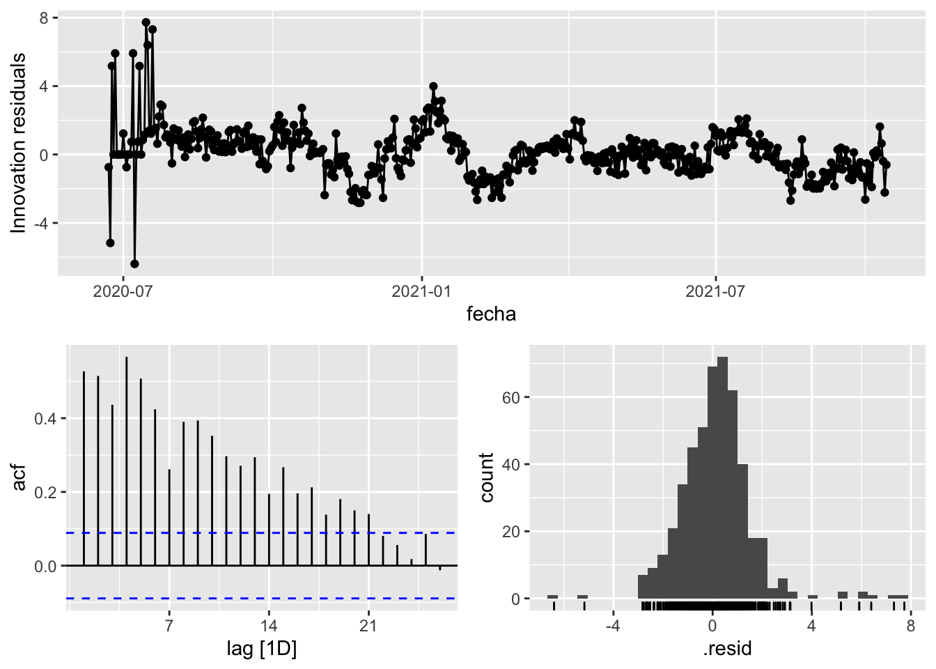
fit_model %>%
      select(arima_at1) %>%
      gg_tsresiduals()
fit_model %>%
      select(arima_at2) %>%
      gg_tsresiduals()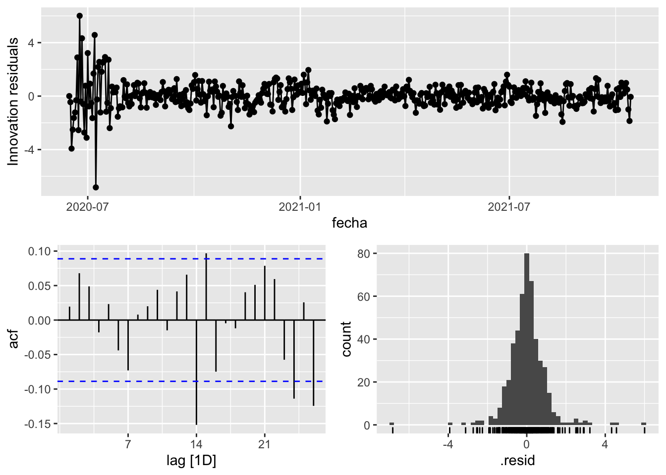
augment(fit_model) %>%
      features(.innov, ljung_box, lag=7)
# A tibble: 3 × 4
provincia .model lb_stat lb_pvalue
<chr> <chr> <dbl> <dbl>
1 Sevilla arima_at1 8.72 0.274
2 Sevilla arima_at2 7.65 0.365
3 Sevilla Snaive 757. 0 augment(fit_model) %>%
features(.innov, ljung_box, lag=14)# A tibble: 3 × 4
provincia .model lb_stat lb_pvalue
<chr> <chr> <dbl> <dbl>
1 Sevilla arima_at1 24.5 0.0402
2 Sevilla arima_at2 23.6 0.0511
3 Sevilla Snaive 1110. 0 augment(fit_model) %>%
features(.innov, ljung_box, lag=21)# A tibble: 3 × 4
provincia .model lb_stat lb_pvalue
<chr> <chr> <dbl> <dbl>
1 Sevilla arima_at1 37.4 0.0151
2 Sevilla arima_at2 36.6 0.0189
3 Sevilla Snaive 1235. 0 augment(fit_model) %>%
features(.innov, ljung_box, lag=90)# A tibble: 3 × 4
provincia .model lb_stat lb_pvalue
<chr> <chr> <dbl> <dbl>
1 Sevilla arima_at1 103. 0.161
2 Sevilla arima_at2 102. 0.179
3 Sevilla Snaive 1692. 0 # Significant spikes out of 30 is still consistent with white noise
# To be sure, use a Ljung-Box test, which has a large p-value, confirming that
# the residuals are similar to white noise.
# Note that the alternative models also passed this test.
#
# Forecast
fc_h7 <- fabletools::forecast(fit_model, h = 7)
fc_h14 <- fabletools::forecast(fit_model, h = 14)
fc_h21 <- fabletools::forecast(fit_model, h = 21)
fc_h90 <- fabletools::forecast(fit_model, h = 90)7 days
# Plots
fc_h7 %>%
      autoplot(
            data_sevilla_test %>%
                  filter(fecha <= as.Date("2021-10-14", format = "%Y-%m-%d")+days(9))
      ) +
      labs(y = "Nº cases", title = "Sevilla - forecast h7")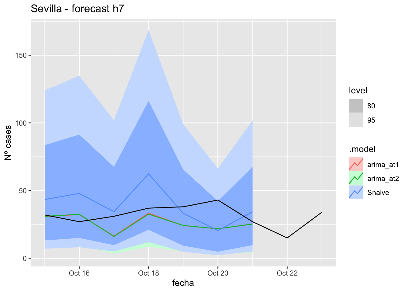
fc_h7 %>%
      autoplot(
            data_sevilla %>%
                  filter(fecha <= as.Date("2021-10-14", format = "%Y-%m-%d")+days(9) &
                               fecha > as.Date("2021-07-01", format = "%Y-%m-%d"))
      ) +
      labs(y = "Nº cases", title = "Sevilla - forecast h7")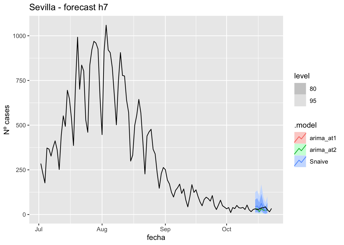
# Accuracy
fabletools::accuracy(fc_h7, data_sevilla)
# A tibble: 3 × 11
.model provincia .type ME RMSE MAE MPE MAPE MASE RMSSE ACF1
<chr> <chr> <chr> <dbl> <dbl> <dbl> <dbl> <dbl> <dbl> <dbl> <dbl>
1 arima_at1 Sevilla Test 7.30 11.4 8.80 19.1 24.7 0.0870 0.0721 -0.0998
2 arima_at2 Sevilla Test 7.38 11.4 8.93 19.3 25.1 0.0883 0.0725 -0.0852
3 Snaive Sevilla Test -5.85 16.0 13.7 -22.0 40.6 0.135 0.102 0.031014 days
# Plots
fc_h14 %>%
      autoplot(
            data_sevilla_test %>%
                  filter(fecha <= as.Date("2021-10-14", format = "%Y-%m-%d")+days(16))
      ) +
      labs(y = "Nº cases", title = "Sevilla - forecast h14")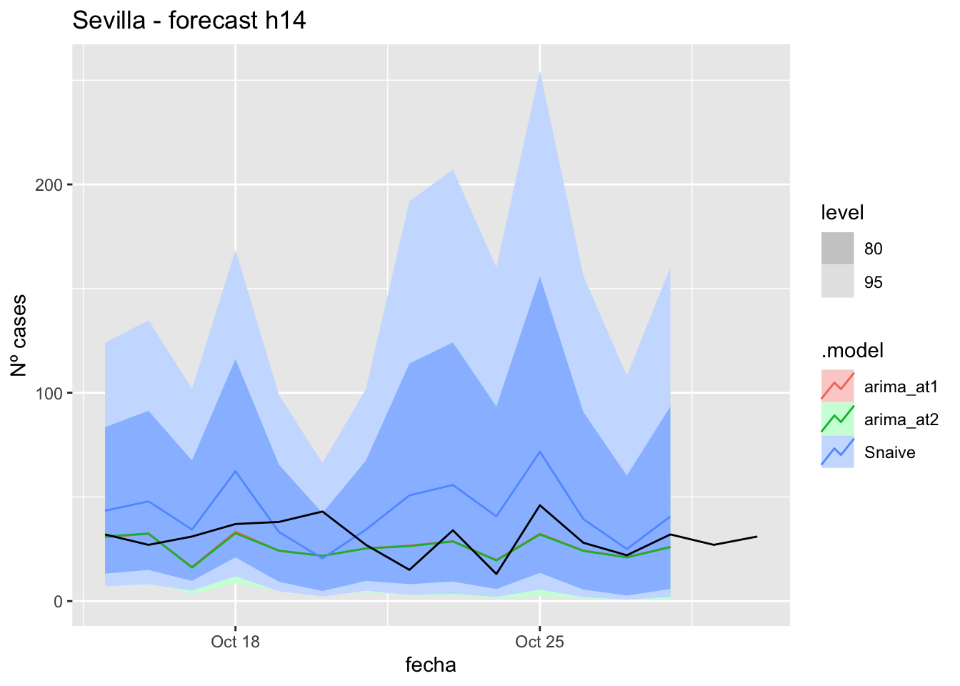
fc_h14 %>%
      autoplot(
            data_sevilla %>%
                  filter(fecha <= as.Date("2021-10-14", format = "%Y-%m-%d")+days(16) &
                               fecha > as.Date("2021-07-01", format = "%Y-%m-%d"))
      ) +
      labs(y = "Nº cases", title = "Sevilla - forecast h14")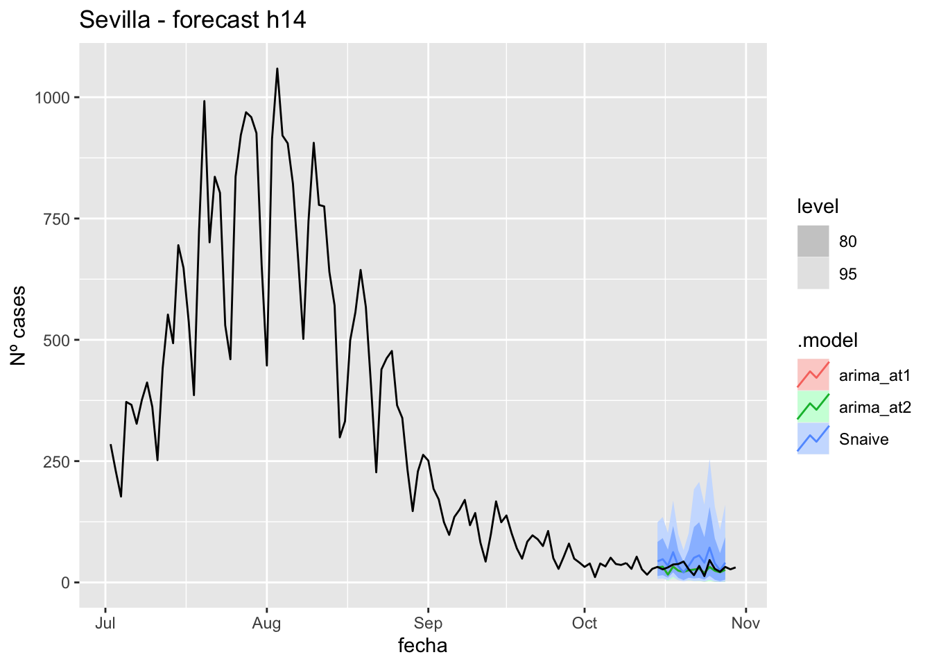
# Accuracy
fabletools::accuracy(fc_h14, data_sevilla)
# A tibble: 3 × 11
.model provincia .type ME RMSE MAE MPE MAPE MASE RMSSE ACF1
<chr> <chr> <chr> <dbl> <dbl> <dbl> <dbl> <dbl> <dbl> <dbl> <dbl>
1 arima_a… Sevilla Test 4.45 9.82 7.83 6.10 27.4 0.0774 0.0623 -0.0579
2 arima_a… Sevilla Test 4.58 9.88 7.91 6.63 27.5 0.0782 0.0626 -0.0509
3 Snaive Sevilla Test -12.5 19.3 16.4 -57.6 66.9 0.162 0.122 0.275 21 days
# Plots
fc_h21 %>%
      autoplot(
            data_sevilla_test %>%
                  filter(fecha <= as.Date("2021-10-14", format = "%Y-%m-%d")+days(23))
      ) +
      labs(y = "Nº cases", title = "Sevilla - forecast h21")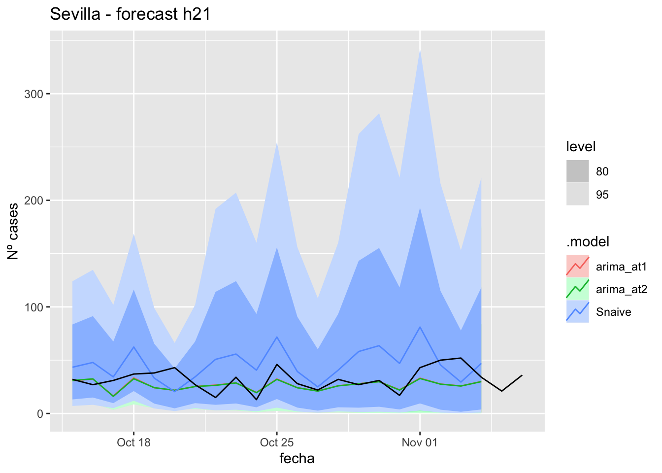
fc_h21 %>%
      autoplot(
            data_sevilla %>%
                  filter(fecha <= as.Date("2021-10-14", format = "%Y-%m-%d")+days(23) &
                               fecha > as.Date("2021-07-01", format = "%Y-%m-%d"))
      ) +
      labs(y = "Nº cases", title = "Sevilla - forecast h21")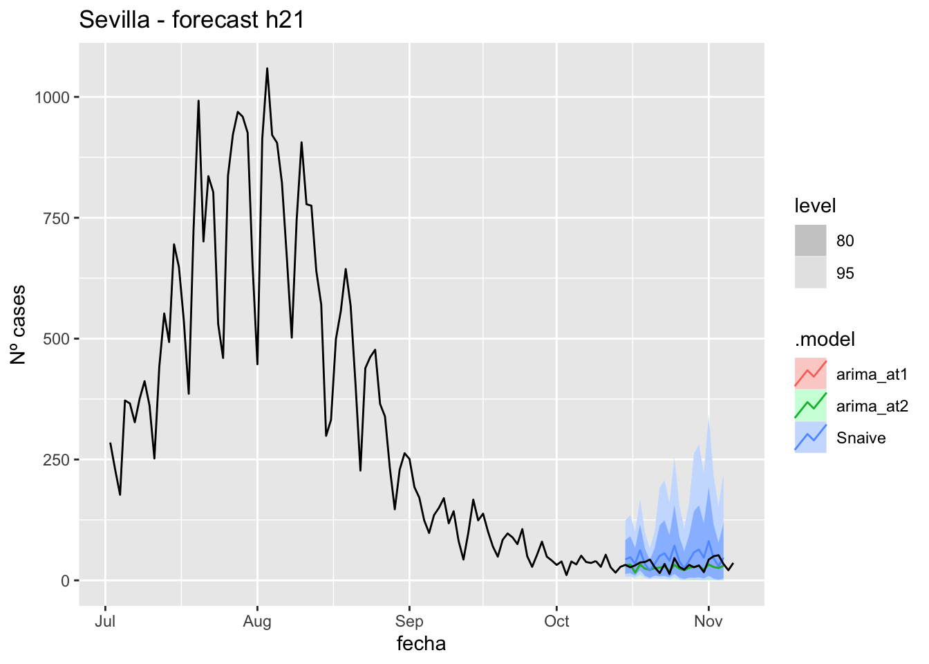
# Accuracy
fabletools::accuracy(fc_h21, data_sevilla)
# A tibble: 3 × 11
.model provincia .type ME RMSE MAE MPE MAPE MASE RMSSE ACF1
<chr> <chr> <chr> <dbl> <dbl> <dbl> <dbl> <dbl> <dbl> <dbl> <dbl>
1 arima_at1 Sevilla Test 5.70 11.3 8.54 8.79 26.3 0.0844 0.0716 0.183
2 arima_at2 Sevilla Test 5.84 11.4 8.61 9.32 26.3 0.0850 0.0720 0.187
3 Snaive Sevilla Test -13.9 22.1 19.1 -60.8 72.0 0.189 0.140 0.32790 days
# Plots
fc_h90 %>%
      autoplot(
            data_sevilla_test %>%
                  filter(fecha <= as.Date("2021-10-14", format = "%Y-%m-%d")+days(92))
      ) +
      labs(y = "Nº cases", title = "Sevilla - forecast h90")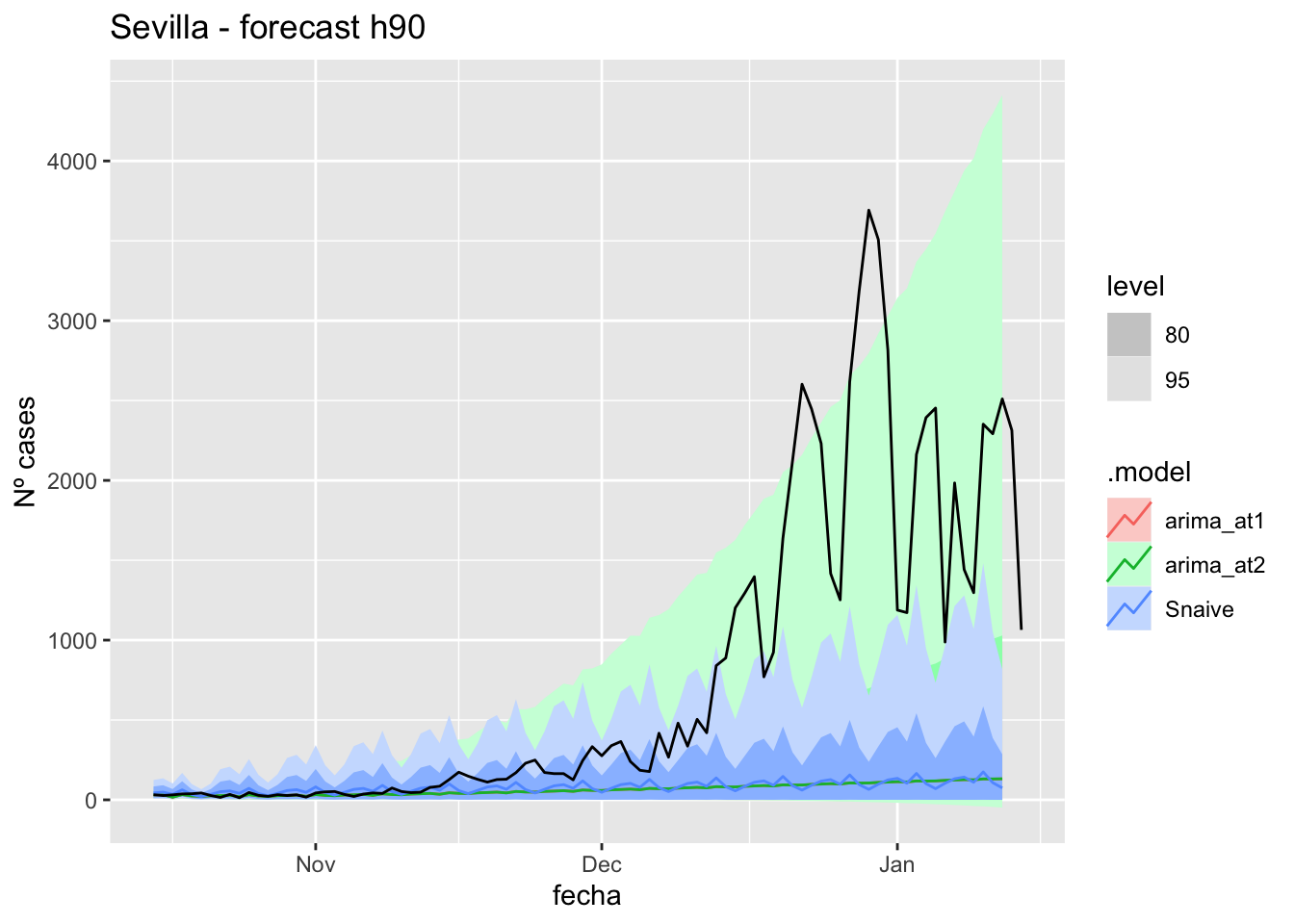
fc_h90 %>%
      autoplot(
            data_sevilla %>%
                  filter(fecha <= as.Date("2021-10-14", format = "%Y-%m-%d")+days(92) &
                               fecha > as.Date("2021-07-01", format = "%Y-%m-%d"))
      ) +
      labs(y = "Nº cases", title = "Sevilla - forecast h90")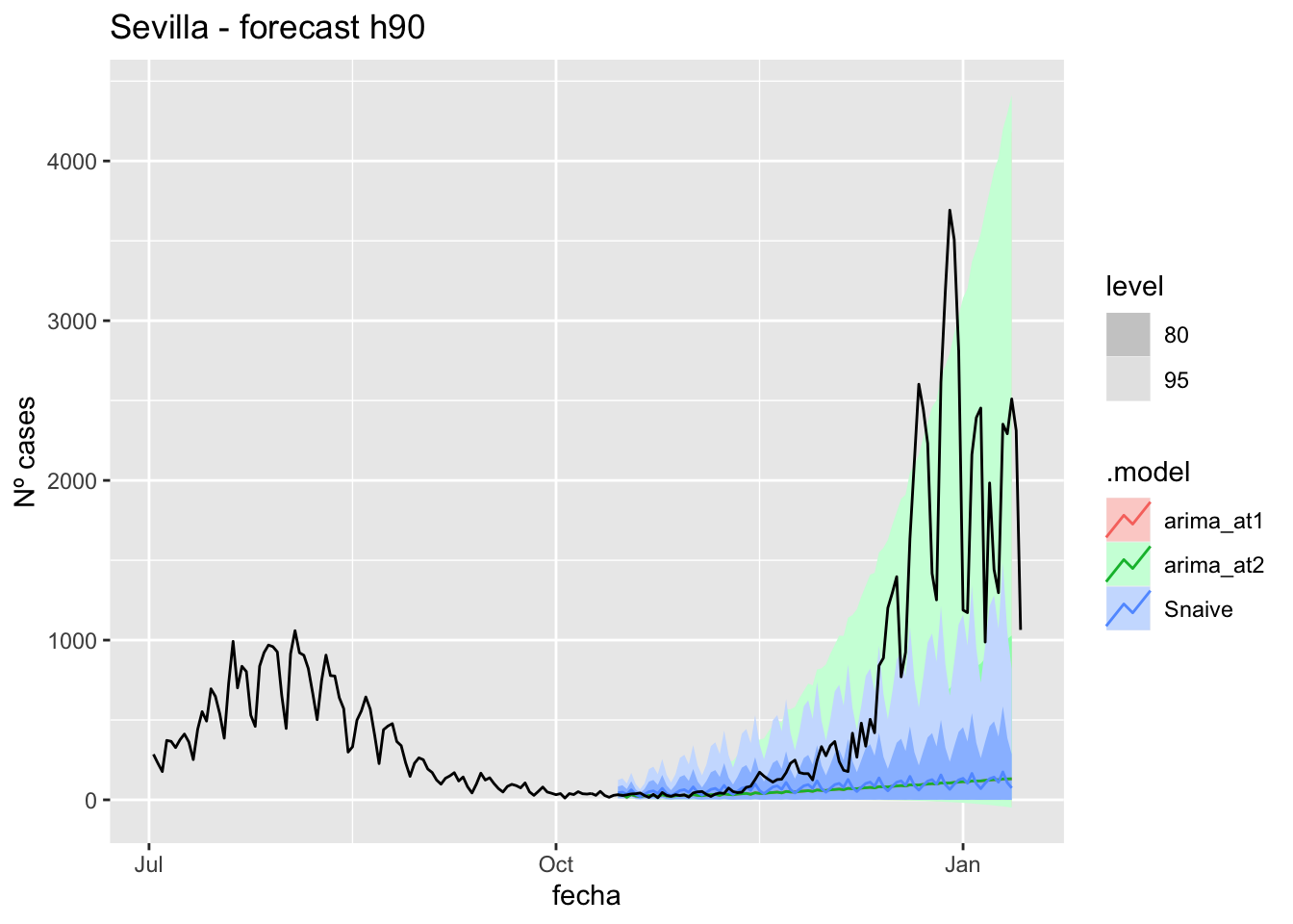
# Accuracy
fabletools::accuracy(fc_h90, data_sevilla)
# A tibble: 3 × 11
.model provincia .type ME RMSE MAE MPE MAPE MASE RMSSE ACF1
<chr> <chr> <chr> <dbl> <dbl> <dbl> <dbl> <dbl> <dbl> <dbl> <dbl>
1 arima_at1 Sevilla Test 681. 1161. 682. 59.5 64.8 6.74 7.36 0.891
2 arima_at2 Sevilla Test 681. 1161. 682. 59.7 64.8 6.74 7.36 0.891
3 Snaive Sevilla Test 665. 1161. 677. 31.7 74.6 6.69 7.36 0.892End of sixth epidemiological period
We are going to keep train the model with data as of June 14th which is considered the beginning of the second epidemiological period in Spain. There are two reasons.
But, instead of predict the last wave, we are going to predict the deleration of infections as to 31 jan 2022.
Asturias
data_asturias <- covid_data %>%
      filter(provincia == "Asturias") %>%
      filter(fecha > as.Date("2020-06-14", format = "%Y-%m-%d")) %>%
      select(provincia, fecha, num_casos, num_hosp, tmed,mob_grocery_pharmacy, mob_parks,
             mob_residential, mob_retail_recreation, mob_transit_stations, mob_workplaces, mob_flujo) %>%
      drop_na(-mob_flujo) %>%
      as_tsibble(key = provincia, index = fecha)
data_asturias
# A tsibble: 653 x 12 [1D]
# Key: provincia [1]
provincia fecha num_casos num_hosp tmed mob_grocery_pharmacy mob_parks
<chr> <date> <dbl> <dbl> <dbl> <dbl> <dbl>
1 Asturias 2020-06-15 0 0 16 -6 39
2 Asturias 2020-06-16 1 0 15.6 -6 7
3 Asturias 2020-06-17 0 0 15.6 -7 20
4 Asturias 2020-06-18 0 0 15.1 -4 68
5 Asturias 2020-06-19 0 0 14.8 -4 52
6 Asturias 2020-06-20 0 0 16.8 -10 71
7 Asturias 2020-06-21 0 0 18.2 -5.5 46
8 Asturias 2020-06-22 0 0 18.2 -1 99
9 Asturias 2020-06-23 0 0 20 -2 129
10 Asturias 2020-06-24 0 0 18.2 -9 63
# … with 643 more rows, and 5 more variables: mob_residential <dbl>,
# mob_retail_recreation <dbl>, mob_transit_stations <dbl>,
# mob_workplaces <dbl>, mob_flujo <dbl>data_asturias_train <- data_asturias %>%
filter(fecha <= as.Date("2022-01-31", format = "%Y-%m-%d"))
summary(data_asturias_train$fecha) Min. 1st Qu. Median Mean 3rd Qu. Max.
"2020-06-15" "2020-11-10" "2021-04-08" "2021-04-08" "2021-09-04" "2022-01-31" data_asturias_test <- data_asturias %>%
filter(fecha > as.Date("2022-01-31", format = "%Y-%m-%d"))
summary(data_asturias_test$fecha) Min. 1st Qu. Median Mean 3rd Qu. Max.
"2022-02-01" "2022-02-15" "2022-03-01" "2022-03-01" "2022-03-15" "2022-03-29" lambda_asturias <- data_asturias %>%
features(num_casos, features = guerrero) %>%
pull(lambda_guerrero)
fit_model <- data_asturias_train %>%
model(
arima_at1 = ARIMA(box_cox(num_casos, lambda_asturias)),
arima_at2 = ARIMA(box_cox(num_casos, lambda_asturias),
stepwise = FALSE, approx = FALSE),
Snaive = SNAIVE(box_cox(num_casos, lambda_asturias))
)
# Show and report model
fit_model# A mable: 1 x 4
# Key: provincia [1]
provincia arima_at1 arima_at2 Snaive
<chr> <model> <model> <model>
1 Asturias <ARIMA(3,1,1)(2,0,0)[7]> <ARIMA(0,1,1)(1,0,1)[7]> <SNAIVE>glance(fit_model)# A tibble: 3 × 9
provincia .model sigma2 log_lik AIC AICc BIC ar_roots ma_roots
<chr> <chr> <dbl> <dbl> <dbl> <dbl> <dbl> <list> <list>
1 Asturias arima_at1 0.917 -816. 1646. 1646. 1677. <cpl [17]> <cpl [1]>
2 Asturias arima_at2 0.894 -811. 1629. 1629. 1647. <cpl [7]> <cpl [8]>
3 Asturias Snaive 2.53 NA NA NA NA <NULL> <NULL> fit_model %>%
pivot_longer(-provincia,
names_to = ".model",
values_to = "orders") %>%
left_join(glance(fit_model), by = c("provincia", ".model")) %>%
arrange(AICc) %>%
select(.model:BIC)# A mable: 3 x 7
# Key: .model [3]
.model orders sigma2 log_lik AIC AICc BIC
<chr> <model> <dbl> <dbl> <dbl> <dbl> <dbl>
1 arima_at2 <ARIMA(0,1,1)(1,0,1)[7]> 0.894 -811. 1629. 1629. 1647.
2 arima_at1 <ARIMA(3,1,1)(2,0,0)[7]> 0.917 -816. 1646. 1646. 1677.
3 Snaive <SNAIVE> 2.53 NA NA NA NA # We use a Ljung-Box test >> large p-value, confirms residuals are similar / considered to white noise
fit_model %>%
select(Snaive) %>%
gg_tsresiduals()
fit_model %>%
select(arima_at1) %>%
gg_tsresiduals()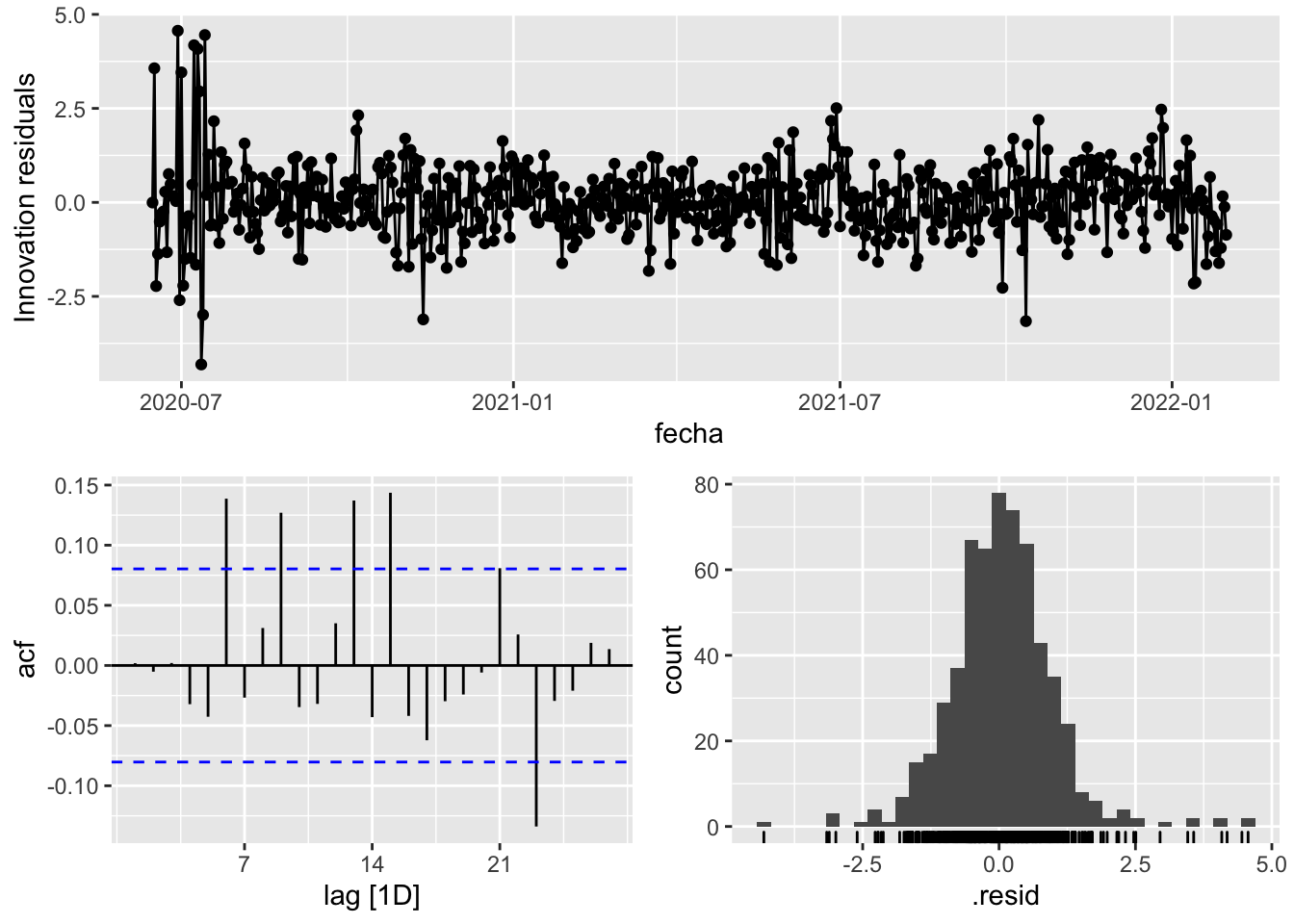
fit_model %>%
select(arima_at2) %>%
gg_tsresiduals()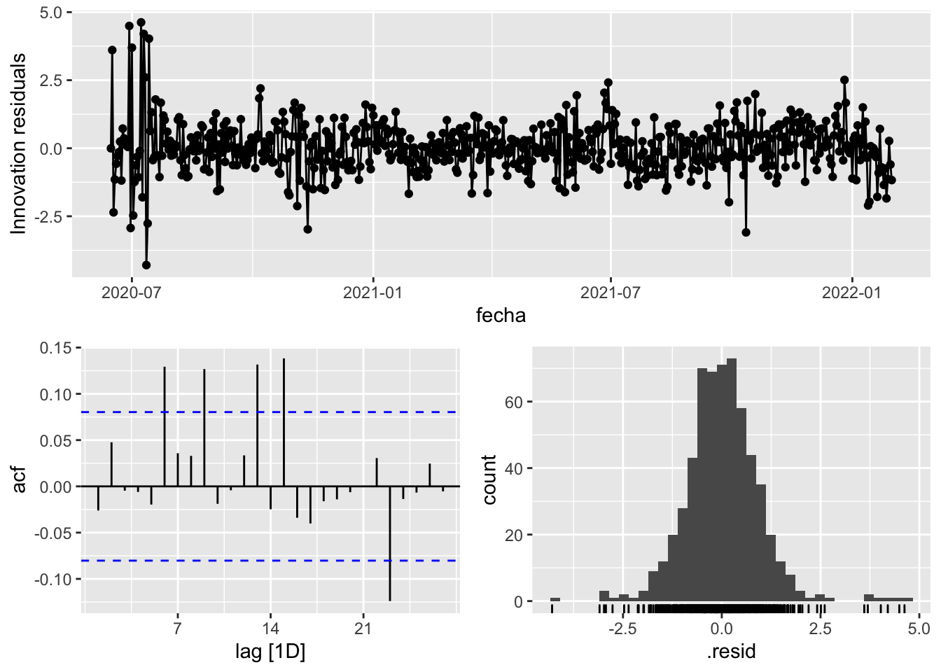
augment(fit_model) %>%
features(.innov, ljung_box, lag=7)# A tibble: 3 × 4
provincia .model lb_stat lb_pvalue
<chr> <chr> <dbl> <dbl>
1 Asturias arima_at1 13.8 0.0551
2 Asturias arima_at2 12.9 0.0743
3 Asturias Snaive 981. 0 augment(fit_model) %>%
features(.innov, ljung_box, lag=14)# A tibble: 3 × 4
provincia .model lb_stat lb_pvalue
<chr> <chr> <dbl> <dbl>
1 Asturias arima_at1 38.9 0.000378
2 Asturias arima_at2 35.2 0.00137
3 Asturias Snaive 1393. 0 augment(fit_model) %>%
features(.innov, ljung_box, lag=21)# A tibble: 3 × 4
provincia .model lb_stat lb_pvalue
<chr> <chr> <dbl> <dbl>
1 Asturias arima_at1 60.0 0.0000128
2 Asturias arima_at2 49.0 0.000509
3 Asturias Snaive 1470. 0 augment(fit_model) %>%
features(.innov, ljung_box, lag=57)# A tibble: 3 × 4
provincia .model lb_stat lb_pvalue
<chr> <chr> <dbl> <dbl>
1 Asturias arima_at1 101. 0.000286
2 Asturias arima_at2 78.6 0.0304
3 Asturias Snaive 1527. 0 # Significant spikes out of 30 is still consistent with white noise
# To be sure, use a Ljung-Box test, which has a large p-value, confirming that
# the residuals are similar to white noise.
# Note that the alternative models also passed this test.
#
# Forecast
fc_h7 <- fabletools::forecast(fit_model, h = 7)
fc_h14 <- fabletools::forecast(fit_model, h = 14)
fc_h21 <- fabletools::forecast(fit_model, h = 21)
fc_h90 <- fabletools::forecast(fit_model, h = 57)7 days
# Plots
fc_h7 %>%
autoplot(
data_asturias_test %>%
filter(fecha <= as.Date("2022-01-31", format = "%Y-%m-%d")+days(9))
) +
labs(y = "Nº cases", title = "Asturias - forecast h7")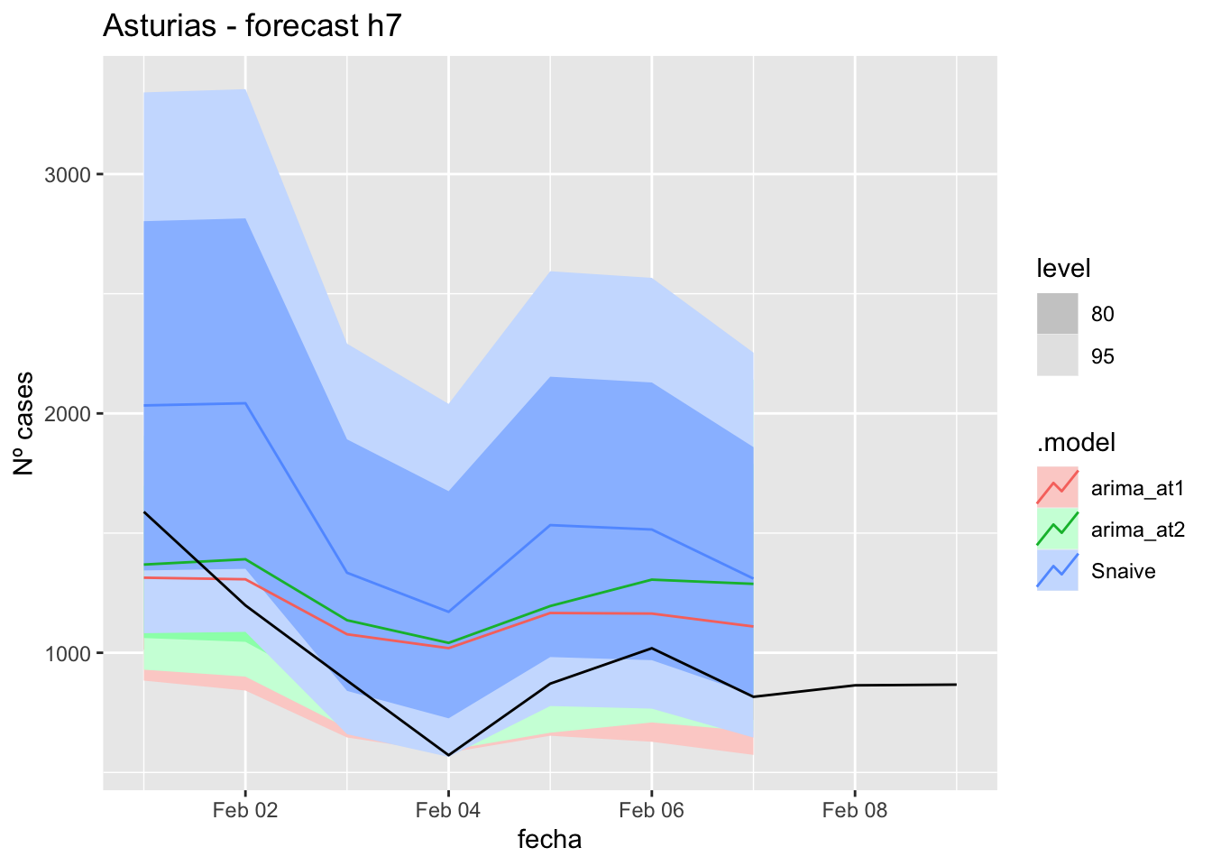
fc_h7 %>%
autoplot(
data_asturias %>%
filter(fecha <= as.Date("2022-01-31", format = "%Y-%m-%d")+days(9) &
fecha > as.Date("2021-12-01", format = "%Y-%m-%d"))
) +
labs(y = "Nº cases", title = "Asturias - forecast h7")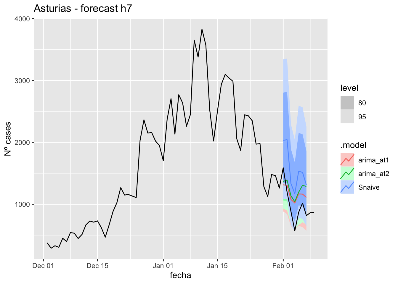
# Accuracy
fabletools::accuracy(fc_h7, data_asturias)# A tibble: 3 × 11
.model provincia .type ME RMSE MAE MPE MAPE MASE RMSSE ACF1
<chr> <chr> <chr> <dbl> <dbl> <dbl> <dbl> <dbl> <dbl> <dbl> <dbl>
1 arima_at1 Asturias Test -173. 272. 251. -25.1 30.1 2.60 1.24 0.192
2 arima_at2 Asturias Test -254. 334. 317. -33.7 37.7 3.27 1.52 0.162
3 Snaive Asturias Test -570. 586. 570. -62.8 62.8 5.89 2.66 -0.55014 days
# Plots
fc_h14 %>%
autoplot(
data_asturias_test %>%
filter(fecha <= as.Date("2022-01-31", format = "%Y-%m-%d")+days(16))
) +
labs(y = "Nº cases", title = "Asturias - forecast h14")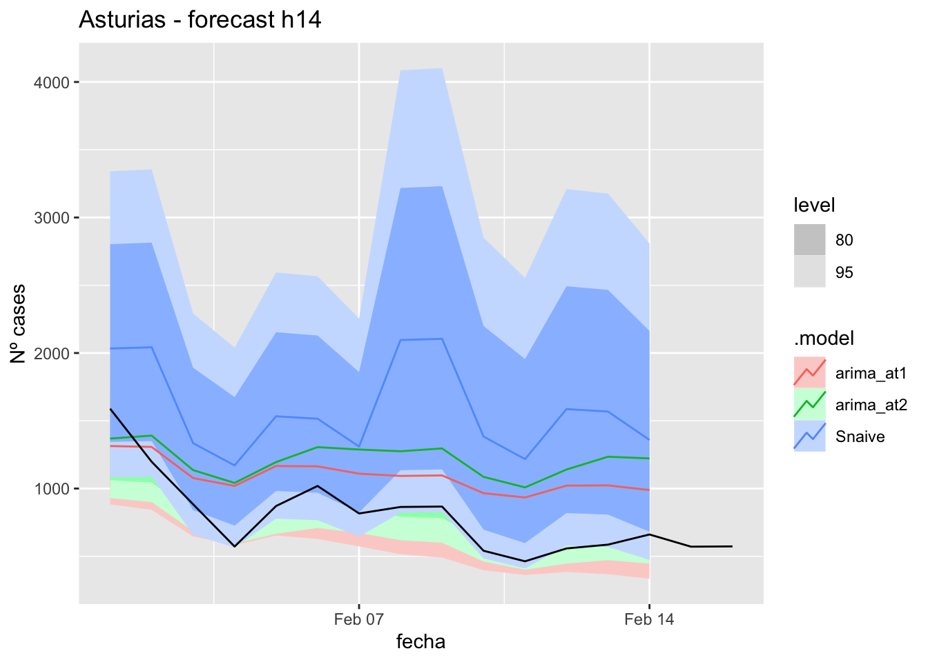
fc_h14 %>%
autoplot(
data_asturias %>%
filter(fecha <= as.Date("2022-01-31", format = "%Y-%m-%d")+days(16) &
fecha > as.Date("2021-12-01", format = "%Y-%m-%d"))
) +
labs(y = "Nº cases", title = "Asturias - forecast h14")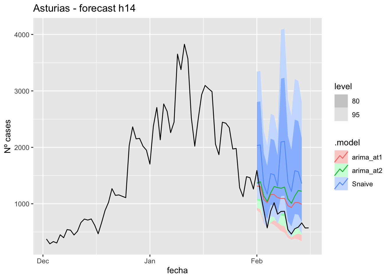
# Accuracy
fabletools::accuracy(fc_h14, data_asturias)# A tibble: 3 × 11
.model provincia .type ME RMSE MAE MPE MAPE MASE RMSSE ACF1
<chr> <chr> <chr> <dbl> <dbl> <dbl> <dbl> <dbl> <dbl> <dbl> <dbl>
1 arima_at1 Asturias Test -271. 332. 310. -44.0 46.5 3.20 1.51 0.372
2 arima_at2 Asturias Test -393. 447. 424. -60.8 62.8 4.38 2.03 0.444
3 Snaive Asturias Test -769. 812. 769. -107. 107. 7.94 3.69 0.29921 days
# Plots
fc_h21 %>%
autoplot(
data_asturias_test %>%
filter(fecha <= as.Date("2022-01-31", format = "%Y-%m-%d")+days(23))
) +
labs(y = "Nº cases", title = "Asturias - forecast h21")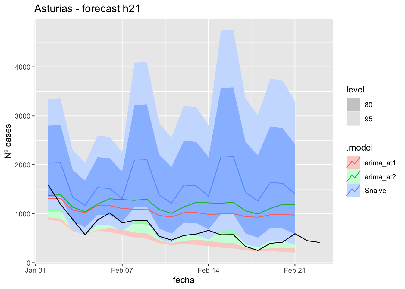
fc_h21 %>%
autoplot(
data_asturias %>%
filter(fecha <= as.Date("2022-01-31", format = "%Y-%m-%d")+days(23) &
fecha > as.Date("2021-12-01", format = "%Y-%m-%d"))
) +
labs(y = "Nº cases", title = "Asturias - forecast h21")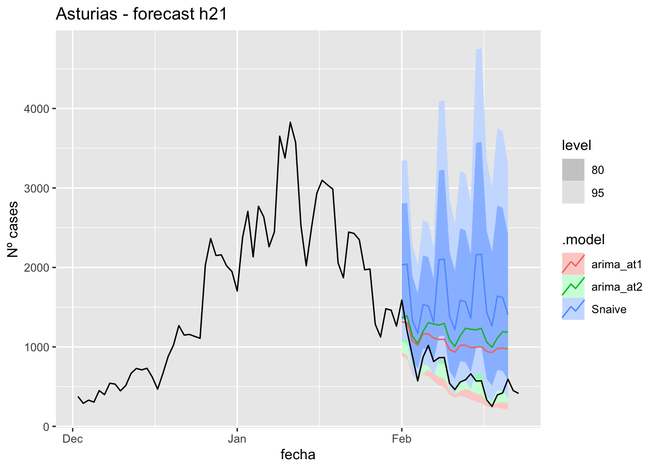
# Accuracy
fabletools::accuracy(fc_h21, data_asturias)# A tibble: 3 × 11
.model provincia .type ME RMSE MAE MPE MAPE MASE RMSSE ACF1
<chr> <chr> <chr> <dbl> <dbl> <dbl> <dbl> <dbl> <dbl> <dbl> <dbl>
1 arima_at1 Asturias Test -355. 411. 381. -74.5 76.1 3.94 1.87 0.532
2 arima_at2 Asturias Test -493. 543. 514. -98.0 99.3 5.31 2.47 0.597
3 Snaive Asturias Test -920. 980. 920. -168. 168. 9.50 4.46 0.43757 days
# Plots
fc_h90 %>%
autoplot(
data_asturias_test %>%
filter(fecha <= as.Date("2022-01-31", format = "%Y-%m-%d")+days(59))
) +
labs(y = "Nº cases", title = "Asturias - forecast h90")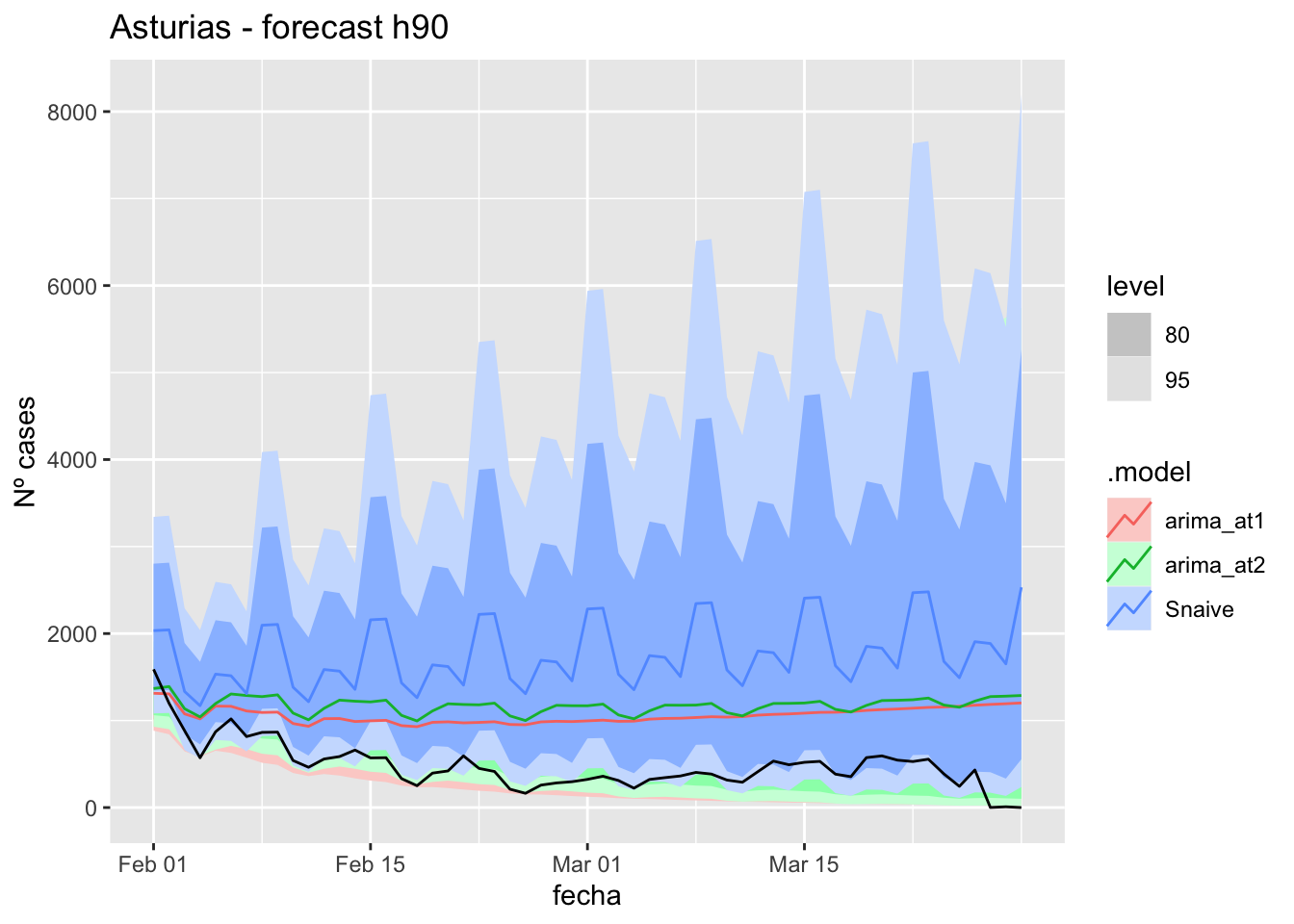
fc_h90 %>%
autoplot(
data_asturias %>%
filter(fecha <= as.Date("2022-01-31", format = "%Y-%m-%d")+days(59) &
fecha > as.Date("2021-12-01", format = "%Y-%m-%d"))
) +
labs(y = "Nº cases", title = "Asturias - forecast h90")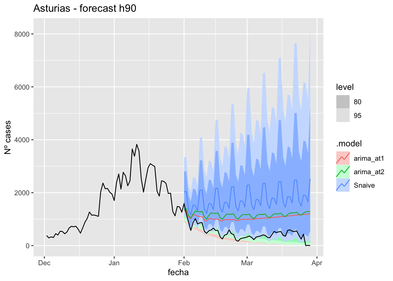
# Accuracy
fabletools::accuracy(fc_h90, data_asturias)# A tibble: 3 × 11
.model provincia .type ME RMSE MAE MPE MAPE MASE RMSSE ACF1
<chr> <chr> <chr> <dbl> <dbl> <dbl> <dbl> <dbl> <dbl> <dbl> <dbl>
1 arima_at1 Asturias Test -579. 631. 589. -Inf Inf 6.09 2.87 0.719
2 arima_at2 Asturias Test -694. 735. 702. -Inf Inf 7.25 3.34 0.714
3 Snaive Asturias Test -1282. 1359. 1282. -Inf Inf 13.3 6.18 0.471Barcelona
data_barcelona <- covid_data %>%
filter(provincia == "Barcelona") %>%
filter(fecha > as.Date("2020-06-14", format = "%Y-%m-%d")) %>%
select(provincia, fecha, num_casos, num_hosp, tmed,mob_grocery_pharmacy, mob_parks,
mob_residential, mob_retail_recreation, mob_transit_stations, mob_workplaces, mob_flujo) %>%
drop_na(-mob_flujo) %>%
as_tsibble(key = provincia, index = fecha)
data_barcelona# A tsibble: 653 x 12 [1D]
# Key: provincia [1]
provincia fecha num_casos num_hosp tmed mob_grocery_pharmacy mob_parks
<chr> <date> <dbl> <dbl> <dbl> <dbl> <dbl>
1 Barcelona 2020-06-15 62 3 21.2 -9 17
2 Barcelona 2020-06-16 66 3 20.8 -10 -16
3 Barcelona 2020-06-17 70 4 20.3 -4 14
4 Barcelona 2020-06-18 68 4 18.8 -8 -6
5 Barcelona 2020-06-19 65 4 20.4 -5 10
6 Barcelona 2020-06-20 53 4 21.8 -12 15
7 Barcelona 2020-06-21 38 1 22.8 -18 18
8 Barcelona 2020-06-22 69 5 23.8 5 24
9 Barcelona 2020-06-23 95 3 23.4 19 28
10 Barcelona 2020-06-24 44 4 23.6 -71 28
# … with 643 more rows, and 5 more variables: mob_residential <dbl>,
# mob_retail_recreation <dbl>, mob_transit_stations <dbl>,
# mob_workplaces <dbl>, mob_flujo <dbl>data_barcelona_train <- data_barcelona %>%
filter(fecha <= as.Date("2022-01-31", format = "%Y-%m-%d"))
summary(data_barcelona_train$fecha) Min. 1st Qu. Median Mean 3rd Qu. Max.
"2020-06-15" "2020-11-10" "2021-04-08" "2021-04-08" "2021-09-04" "2022-01-31" data_barcelona_test <- data_barcelona %>%
filter(fecha > as.Date("2022-01-31", format = "%Y-%m-%d"))
summary(data_barcelona_test$fecha) Min. 1st Qu. Median Mean 3rd Qu. Max.
"2022-02-01" "2022-02-15" "2022-03-01" "2022-03-01" "2022-03-15" "2022-03-29" lambda_Barcelona <- data_barcelona %>%
features(num_casos, features = guerrero) %>%
pull(lambda_guerrero)
fit_model <- data_barcelona_train %>%
model(
arima_at1 = ARIMA(box_cox(num_casos, lambda_Barcelona)),
arima_at2 = ARIMA(box_cox(num_casos, lambda_Barcelona),
stepwise = FALSE, approx = FALSE),
Snaive = SNAIVE(box_cox(num_casos, lambda_Barcelona))
)
# Show and report model
fit_model# A mable: 1 x 4
# Key: provincia [1]
provincia arima_at1 arima_at2 Snaive
<chr> <model> <model> <model>
1 Barcelona <ARIMA(1,0,2)(0,1,1)[7]> <ARIMA(1,0,4)(0,1,1)[7]> <SNAIVE>glance(fit_model)# A tibble: 3 × 9
provincia .model sigma2 log_lik AIC AICc BIC ar_roots ma_roots
<chr> <chr> <dbl> <dbl> <dbl> <dbl> <dbl> <list> <list>
1 Barcelona arima_at1 0.344 -523. 1055. 1055. 1077. <cpl [1]> <cpl [9]>
2 Barcelona arima_at2 0.341 -520. 1053. 1053. 1084. <cpl [1]> <cpl [11]>
3 Barcelona Snaive 1.26 NA NA NA NA <NULL> <NULL> fit_model %>%
pivot_longer(-provincia,
names_to = ".model",
values_to = "orders") %>%
left_join(glance(fit_model), by = c("provincia", ".model")) %>%
arrange(AICc) %>%
select(.model:BIC)# A mable: 3 x 7
# Key: .model [3]
.model orders sigma2 log_lik AIC AICc BIC
<chr> <model> <dbl> <dbl> <dbl> <dbl> <dbl>
1 arima_at2 <ARIMA(1,0,4)(0,1,1)[7]> 0.341 -520. 1053. 1053. 1084.
2 arima_at1 <ARIMA(1,0,2)(0,1,1)[7]> 0.344 -523. 1055. 1055. 1077.
3 Snaive <SNAIVE> 1.26 NA NA NA NA # We use a Ljung-Box test >> large p-value, confirms residuals are similar / considered to white noise
fit_model %>%
select(Snaive) %>%
gg_tsresiduals()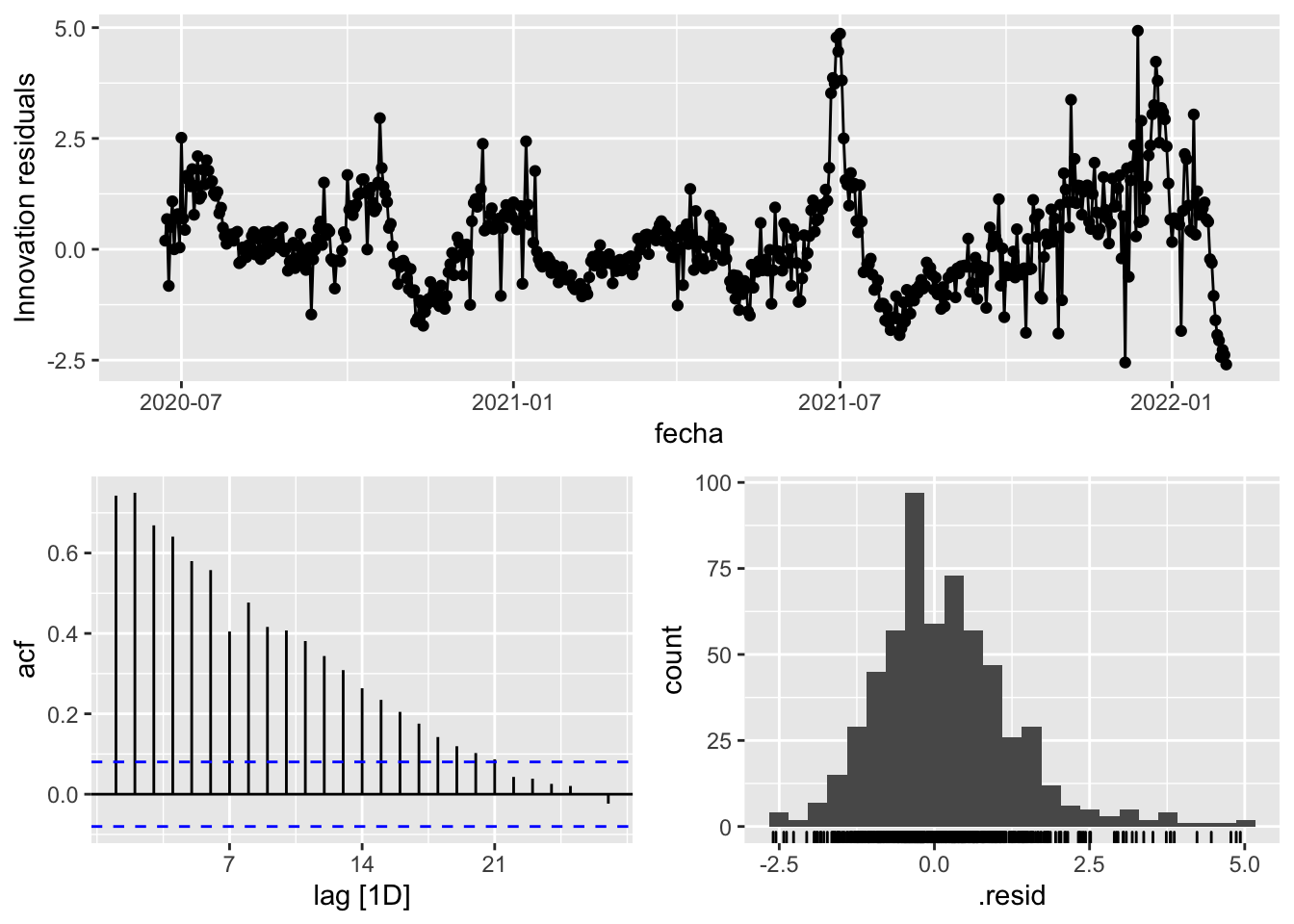
fit_model %>%
select(arima_at1) %>%
gg_tsresiduals()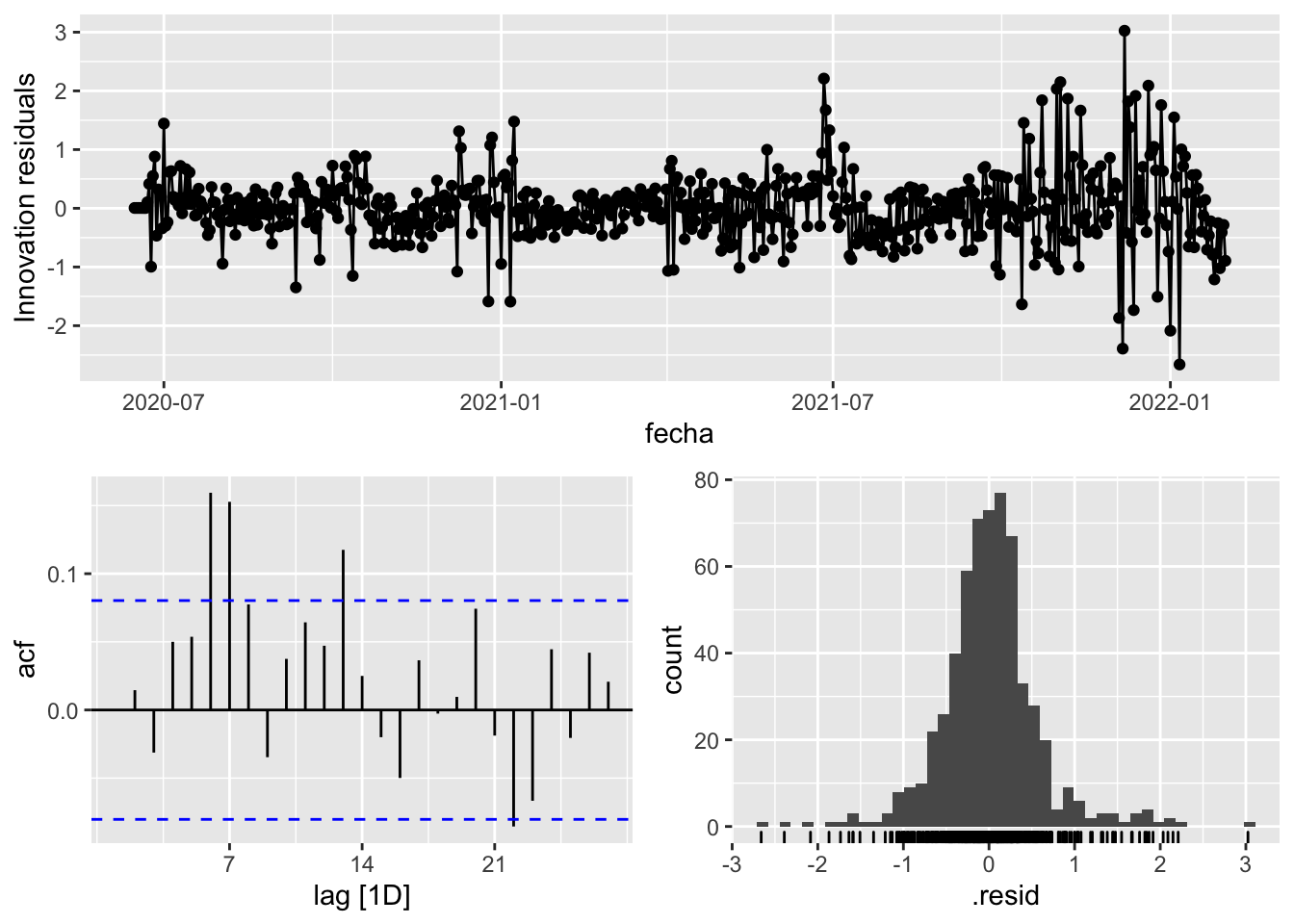
fit_model %>%
select(arima_at2) %>%
gg_tsresiduals()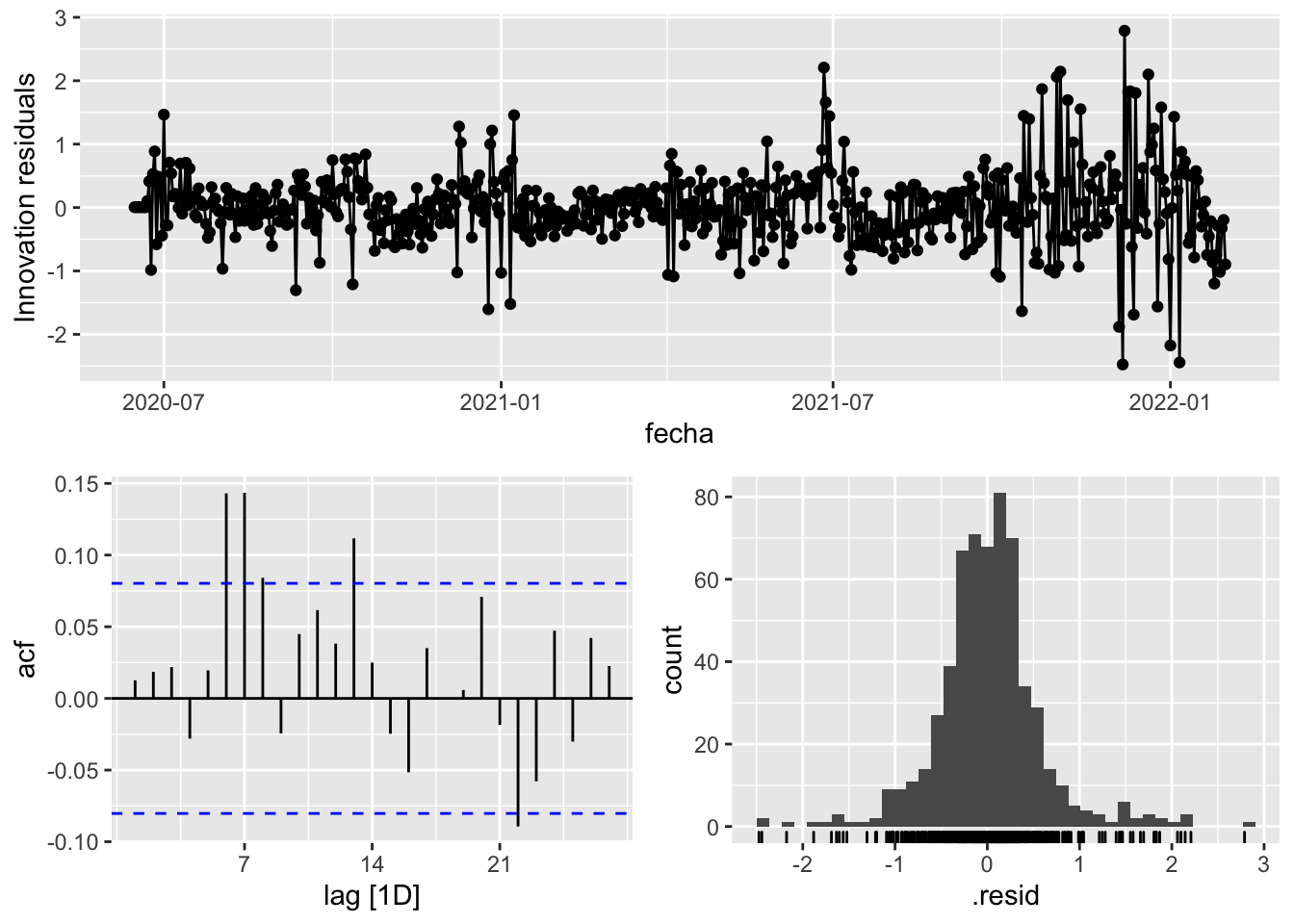
augment(fit_model) %>%
features(.innov, ljung_box, lag=7)# A tibble: 3 × 4
provincia .model lb_stat lb_pvalue
<chr> <chr> <dbl> <dbl>
1 Barcelona arima_at1 33.4 0.0000220
2 Barcelona arima_at2 26.1 0.000480
3 Barcelona Snaive 1654. 0 augment(fit_model) %>%
features(.innov, ljung_box, lag=14)# A tibble: 3 × 4
provincia .model lb_stat lb_pvalue
<chr> <chr> <dbl> <dbl>
1 Barcelona arima_at1 51.3 0.00000363
2 Barcelona arima_at2 43.2 0.0000793
3 Barcelona Snaive 2253. 0 augment(fit_model) %>%
features(.innov, ljung_box, lag=21)# A tibble: 3 × 4
provincia .model lb_stat lb_pvalue
<chr> <chr> <dbl> <dbl>
1 Barcelona arima_at1 57.6 0.0000289
2 Barcelona arima_at2 49.3 0.000455
3 Barcelona Snaive 2362. 0 augment(fit_model) %>%
features(.innov, ljung_box, lag=57)# A tibble: 3 × 4
provincia .model lb_stat lb_pvalue
<chr> <chr> <dbl> <dbl>
1 Barcelona arima_at1 162. 4.59e-12
2 Barcelona arima_at2 153. 9.83e-11
3 Barcelona Snaive 2651. 0 # Significant spikes out of 30 is still consistent with white noise
# To be sure, use a Ljung-Box test, which has a large p-value, confirming that
# the residuals are similar to white noise.
# Note that the alternative models also passed this test.
#
# Forecast
fc_h7 <- fabletools::forecast(fit_model, h = 7)
fc_h14 <- fabletools::forecast(fit_model, h = 14)
fc_h21 <- fabletools::forecast(fit_model, h = 21)
fc_h90 <- fabletools::forecast(fit_model, h = 57)7 days
# Plots
fc_h7 %>%
autoplot(
data_barcelona_test %>%
filter(fecha <= as.Date("2022-01-31", format = "%Y-%m-%d")+days(9))
) +
labs(y = "Nº cases", title = "Barcelona - forecast h7")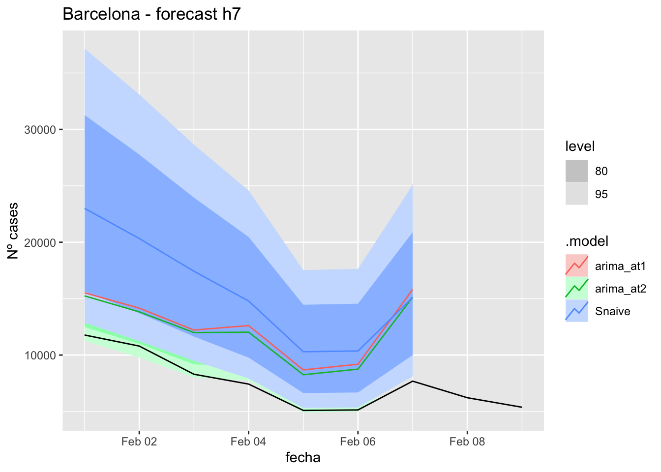
fc_h7 %>%
autoplot(
data_barcelona %>%
filter(fecha <= as.Date("2022-01-31", format = "%Y-%m-%d")+days(9) &
fecha > as.Date("2021-12-01", format = "%Y-%m-%d"))
) +
labs(y = "Nº cases", title = "Barcelona - forecast h7")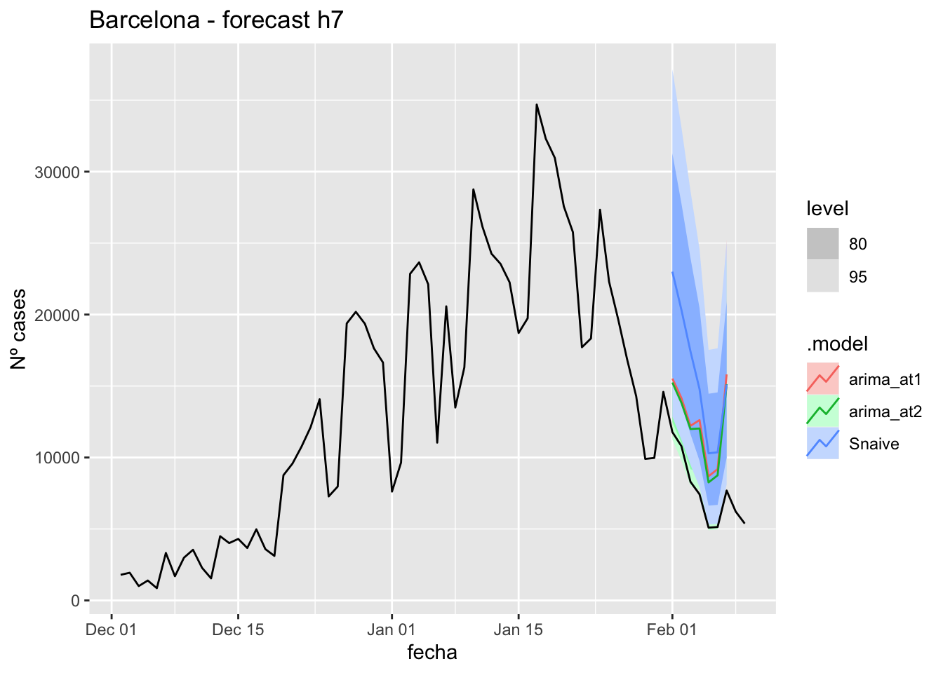
# Accuracy
fabletools::accuracy(fc_h7, data_barcelona)# A tibble: 3 × 11
.model provincia .type ME RMSE MAE MPE MAPE MASE RMSSE ACF1
<chr> <chr> <chr> <dbl> <dbl> <dbl> <dbl> <dbl> <dbl> <dbl> <dbl>
1 arima_at1 Barcelona Test -4569. 4824. 4569. -62.2 62.2 5.74 2.46 -0.0331
2 arima_at2 Barcelona Test -4145. 4383. 4145. -56.2 56.2 5.21 2.24 -0.0435
3 Snaive Barcelona Test -7870. 8139. 7870. -99.0 99.0 9.88 4.16 0.551 14 days
# Plots
fc_h14 %>%
autoplot(
data_barcelona_test %>%
filter(fecha <= as.Date("2022-01-31", format = "%Y-%m-%d")+days(16))
) +
labs(y = "Nº cases", title = "Barcelona - forecast h14")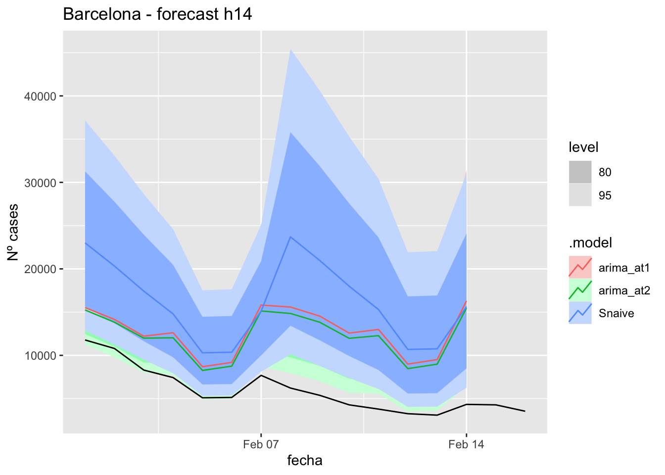
fc_h14 %>%
autoplot(
data_barcelona %>%
filter(fecha <= as.Date("2022-01-31", format = "%Y-%m-%d")+days(16) &
fecha > as.Date("2021-12-01", format = "%Y-%m-%d"))
) +
labs(y = "Nº cases", title = "Barcelona - forecast h14")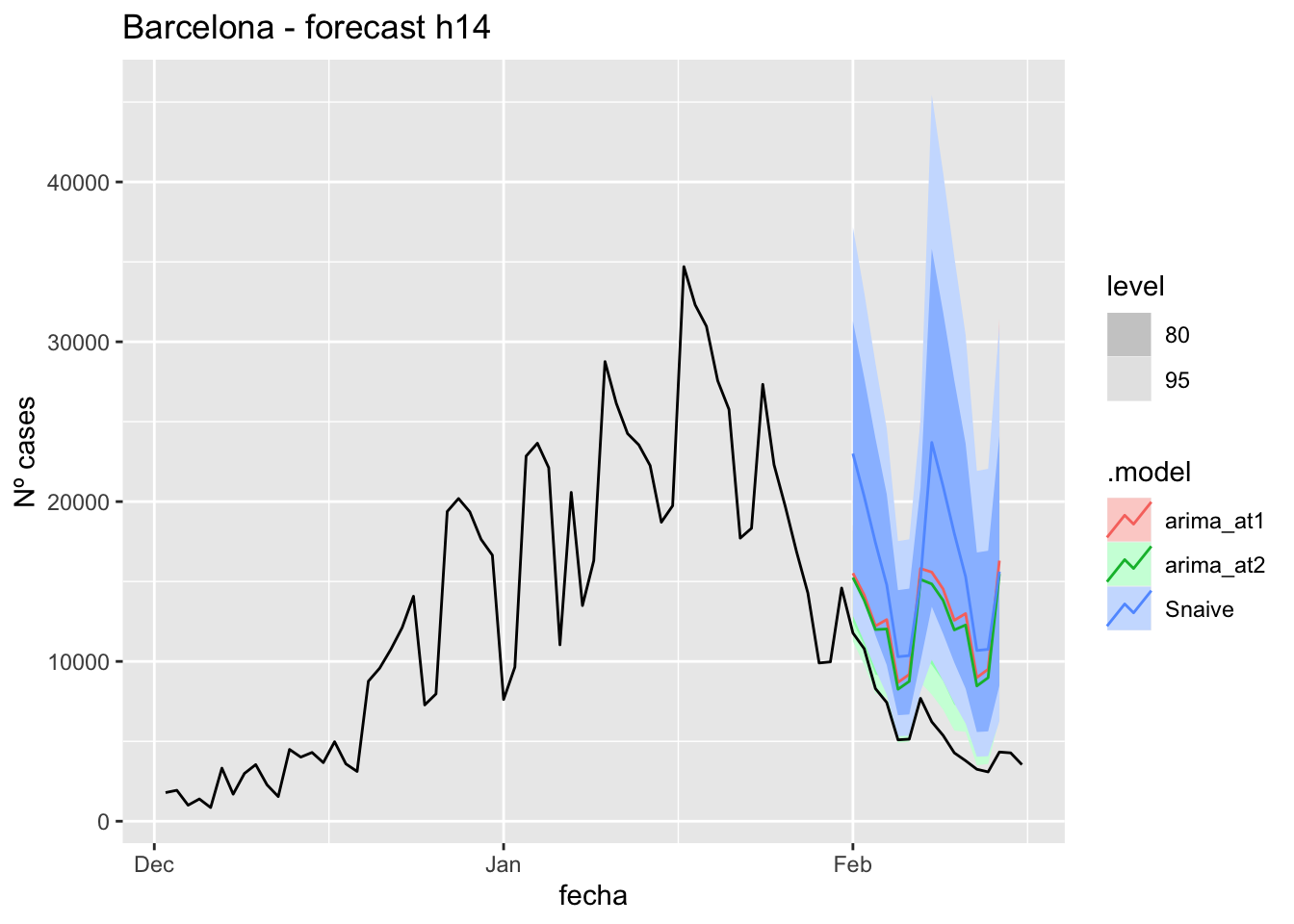
# Accuracy
fabletools::accuracy(fc_h14, data_barcelona)# A tibble: 3 × 11
.model provincia .type ME RMSE MAE MPE MAPE MASE RMSSE ACF1
<chr> <chr> <chr> <dbl> <dbl> <dbl> <dbl> <dbl> <dbl> <dbl> <dbl>
1 arima_at1 Barcelona Test -6582. 7100. 6582. -132. 132. 8.27 3.63 0.471
2 arima_at2 Barcelona Test -6038. 6534. 6038. -122. 122. 7.58 3.34 0.471
3 Snaive Barcelona Test -9985. 10606. 9985. -188. 188. 12.5 5.42 0.54821 days
# Plots
fc_h21 %>%
autoplot(
data_barcelona_test %>%
filter(fecha <= as.Date("2022-01-31", format = "%Y-%m-%d")+days(23))
) +
labs(y = "Nº cases", title = "Barcelona - forecast h21")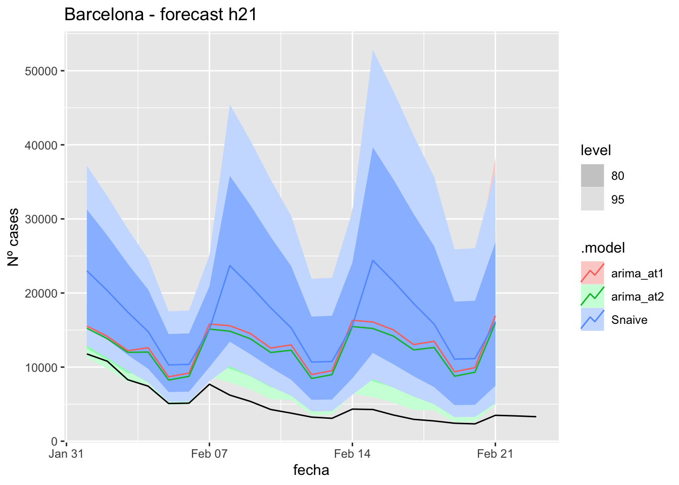
fc_h21 %>%
autoplot(
data_barcelona %>%
filter(fecha <= as.Date("2022-01-31", format = "%Y-%m-%d")+days(23) &
fecha > as.Date("2021-12-01", format = "%Y-%m-%d"))
) +
labs(y = "Nº cases", title = "Barcelona - forecast h21")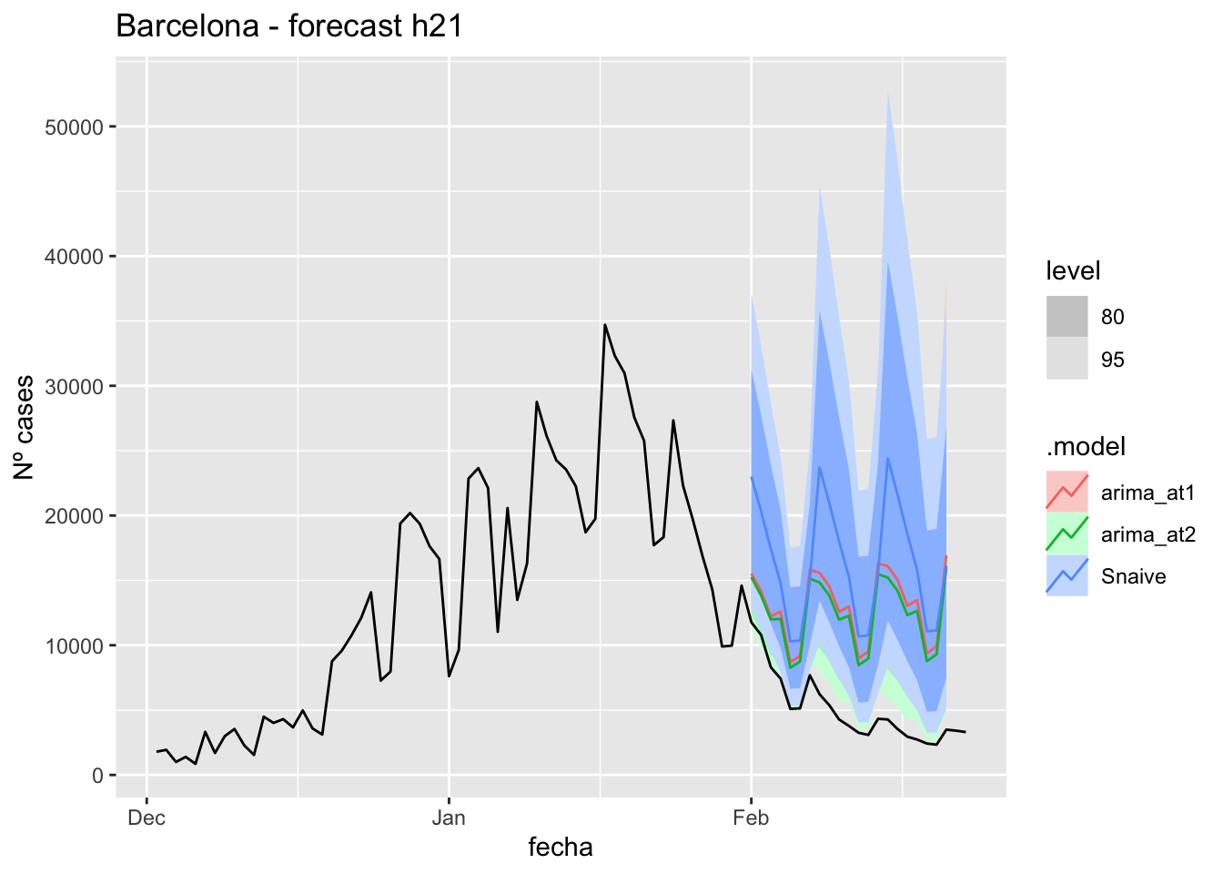
# Accuracy
fabletools::accuracy(fc_h21, data_barcelona)# A tibble: 3 × 11
.model provincia .type ME RMSE MAE MPE MAPE MASE RMSSE ACF1
<chr> <chr> <chr> <dbl> <dbl> <dbl> <dbl> <dbl> <dbl> <dbl> <dbl>
1 arima_at1 Barcelona Test -7823. 8400. 7823. -199. 199. 9.83 4.29 0.573
2 arima_at2 Barcelona Test -7199. 7750. 7199. -184. 184. 9.04 3.96 0.575
3 Snaive Barcelona Test -11275. 12018. 11275. -272. 272. 14.2 6.14 0.60257 days
# Plots
fc_h90 %>%
autoplot(
data_barcelona_test %>%
filter(fecha <= as.Date("2022-01-31", format = "%Y-%m-%d")+days(59))
) +
labs(y = "Nº cases", title = "Barcelona - forecast h90")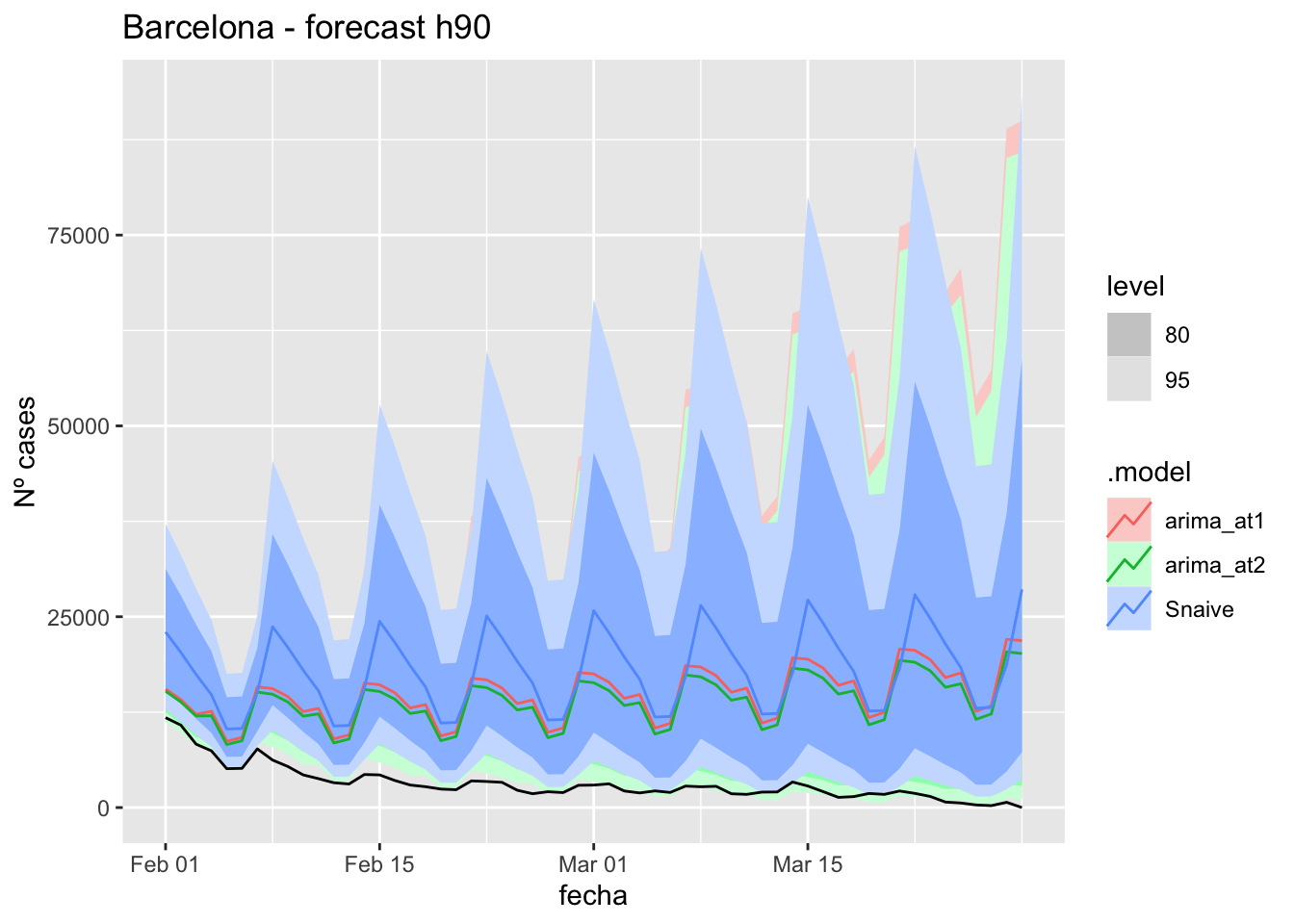
fc_h90 %>%
autoplot(
data_barcelona %>%
filter(fecha <= as.Date("2022-01-31", format = "%Y-%m-%d")+days(59) &
fecha > as.Date("2021-12-01", format = "%Y-%m-%d"))
) +
labs(y = "Nº cases", title = "Barcelona - forecast h90")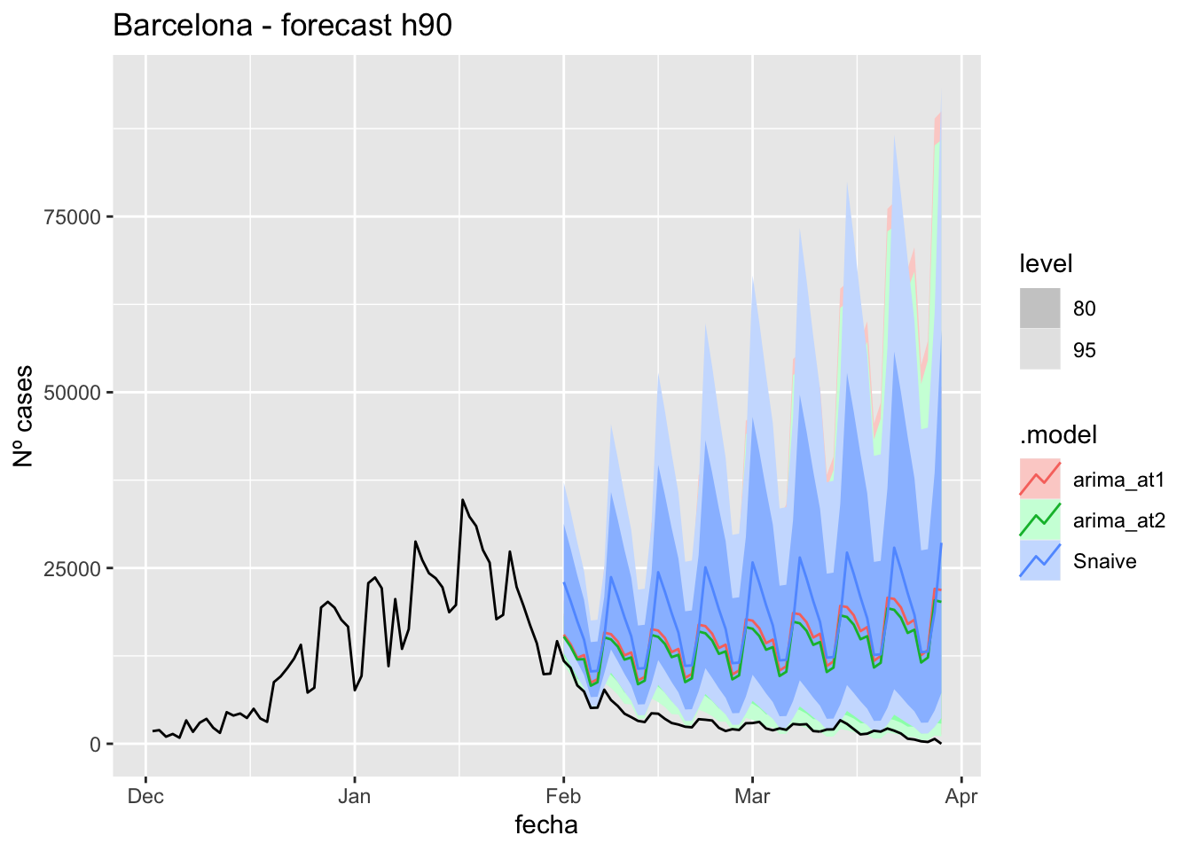
# Accuracy
fabletools::accuracy(fc_h90, data_barcelona)# A tibble: 3 × 11
.model provincia .type ME RMSE MAE MPE MAPE MASE RMSSE ACF1
<chr> <chr> <chr> <dbl> <dbl> <dbl> <dbl> <dbl> <dbl> <dbl> <dbl>
1 arima_at1 Barcelona Test -11642. 12454. 11642. -Inf Inf 14.6 6.36 0.695
2 arima_at2 Barcelona Test -10693. 11449. 10693. -Inf Inf 13.4 5.85 0.691
3 Snaive Barcelona Test -14809. 15796. 14809. -Inf Inf 18.6 8.06 0.592Madrid
data_madrid <- covid_data %>%
filter(provincia == "Madrid") %>%
filter(fecha > as.Date("2020-06-14", format = "%Y-%m-%d")) %>%
select(provincia, fecha, num_casos, num_hosp, tmed,mob_grocery_pharmacy, mob_parks,
mob_residential, mob_retail_recreation, mob_transit_stations, mob_workplaces, mob_flujo) %>%
drop_na(-mob_flujo) %>%
as_tsibble(key = provincia, index = fecha)
data_madrid# A tsibble: 653 x 12 [1D]
# Key: provincia [1]
provincia fecha num_casos num_hosp tmed mob_grocery_pharmacy mob_parks
<chr> <date> <dbl> <dbl> <dbl> <dbl> <dbl>
1 Madrid 2020-06-15 153 10 20.7 -8 34
2 Madrid 2020-06-16 91 16 21 -8 21
3 Madrid 2020-06-17 93 14 20.2 -5 34
4 Madrid 2020-06-18 85 17 21.9 -7 30
5 Madrid 2020-06-19 78 20 22.6 -9 22
6 Madrid 2020-06-20 67 20 23.4 -12 25
7 Madrid 2020-06-21 42 3 25 -13 14
8 Madrid 2020-06-22 60 16 27.3 -8 29
9 Madrid 2020-06-23 68 11 28.4 -9 23
10 Madrid 2020-06-24 49 15 28 -7 22
# … with 643 more rows, and 5 more variables: mob_residential <dbl>,
# mob_retail_recreation <dbl>, mob_transit_stations <dbl>,
# mob_workplaces <dbl>, mob_flujo <dbl>data_madrid_train <- data_madrid %>%
filter(fecha <= as.Date("2022-01-31", format = "%Y-%m-%d"))
summary(data_madrid_train$fecha) Min. 1st Qu. Median Mean 3rd Qu. Max.
"2020-06-15" "2020-11-10" "2021-04-08" "2021-04-08" "2021-09-04" "2022-01-31" data_madrid_test <- data_madrid %>%
filter(fecha > as.Date("2022-01-31", format = "%Y-%m-%d"))
summary(data_madrid_test$fecha) Min. 1st Qu. Median Mean 3rd Qu. Max.
"2022-02-01" "2022-02-15" "2022-03-01" "2022-03-01" "2022-03-15" "2022-03-29" lambda_Madrid <- data_madrid %>%
features(num_casos, features = guerrero) %>%
pull(lambda_guerrero)
fit_model <- data_madrid_train %>%
model(
arima_at1 = ARIMA(box_cox(num_casos, lambda_Madrid)),
arima_at2 = ARIMA(box_cox(num_casos, lambda_Madrid),
stepwise = FALSE, approx = FALSE),
Snaive = SNAIVE(box_cox(num_casos, lambda_Madrid))
)
# Show and report model
fit_model# A mable: 1 x 4
# Key: provincia [1]
provincia arima_at1 arima_at2 Snaive
<chr> <model> <model> <model>
1 Madrid <ARIMA(2,0,2)(0,1,2)[7]> <ARIMA(2,0,2)(0,1,2)[7]> <SNAIVE>glance(fit_model)# A tibble: 3 × 9
provincia .model sigma2 log_lik AIC AICc BIC ar_roots ma_roots
<chr> <chr> <dbl> <dbl> <dbl> <dbl> <dbl> <list> <list>
1 Madrid arima_at1 0.132 -240. 494. 495. 525. <cpl [2]> <cpl [16]>
2 Madrid arima_at2 0.132 -240. 494. 495. 525. <cpl [2]> <cpl [16]>
3 Madrid Snaive 0.412 NA NA NA NA <NULL> <NULL> fit_model %>%
pivot_longer(-provincia,
names_to = ".model",
values_to = "orders") %>%
left_join(glance(fit_model), by = c("provincia", ".model")) %>%
arrange(AICc) %>%
select(.model:BIC)# A mable: 3 x 7
# Key: .model [3]
.model orders sigma2 log_lik AIC AICc BIC
<chr> <model> <dbl> <dbl> <dbl> <dbl> <dbl>
1 arima_at1 <ARIMA(2,0,2)(0,1,2)[7]> 0.132 -240. 494. 495. 525.
2 arima_at2 <ARIMA(2,0,2)(0,1,2)[7]> 0.132 -240. 494. 495. 525.
3 Snaive <SNAIVE> 0.412 NA NA NA NA # We use a Ljung-Box test >> large p-value, confirms residuals are similar / considered to white noise
fit_model %>%
select(Snaive) %>%
gg_tsresiduals()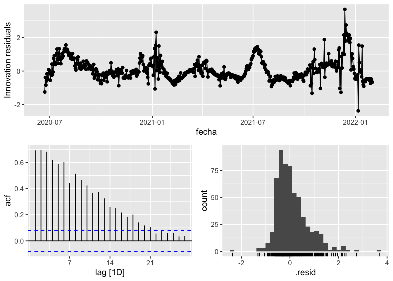
fit_model %>%
select(arima_at1) %>%
gg_tsresiduals()
fit_model %>%
select(arima_at2) %>%
gg_tsresiduals()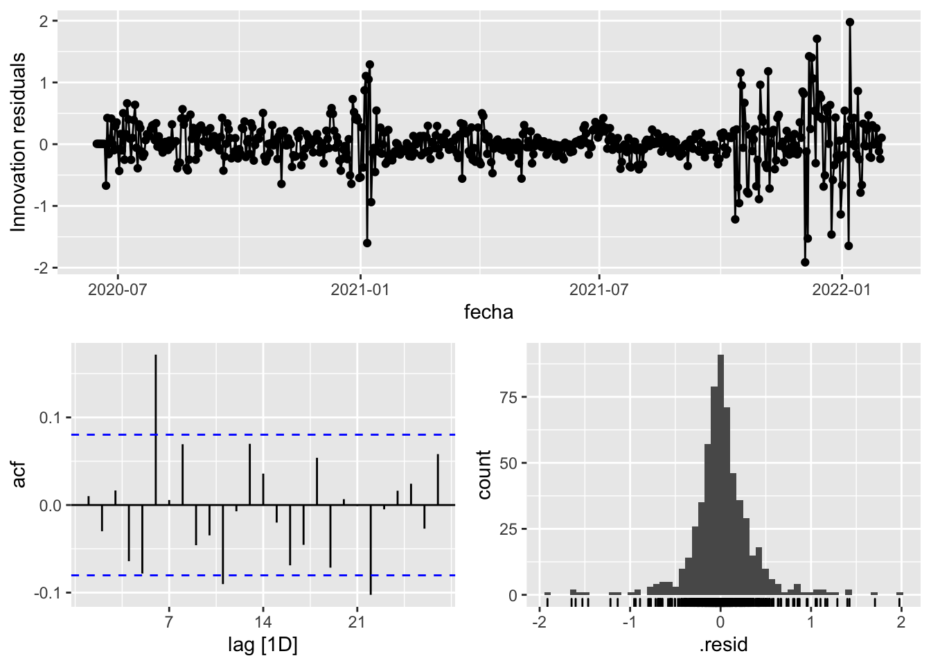
augment(fit_model) %>%
features(.innov, ljung_box, lag=7)# A tibble: 3 × 4
provincia .model lb_stat lb_pvalue
<chr> <chr> <dbl> <dbl>
1 Madrid arima_at1 24.8 0.000838
2 Madrid arima_at2 24.8 0.000838
3 Madrid Snaive 1617. 0 augment(fit_model) %>%
features(.innov, ljung_box, lag=14)# A tibble: 3 × 4
provincia .model lb_stat lb_pvalue
<chr> <chr> <dbl> <dbl>
1 Madrid arima_at1 38.5 0.000443
2 Madrid arima_at2 38.5 0.000443
3 Madrid Snaive 2282. 0 augment(fit_model) %>%
features(.innov, ljung_box, lag=21)# A tibble: 3 × 4
provincia .model lb_stat lb_pvalue
<chr> <chr> <dbl> <dbl>
1 Madrid arima_at1 47.9 0.000718
2 Madrid arima_at2 47.9 0.000718
3 Madrid Snaive 2422. 0 augment(fit_model) %>%
features(.innov, ljung_box, lag=57)# A tibble: 3 × 4
provincia .model lb_stat lb_pvalue
<chr> <chr> <dbl> <dbl>
1 Madrid arima_at1 123. 0.000000995
2 Madrid arima_at2 123. 0.000000995
3 Madrid Snaive 2762. 0 # Significant spikes out of 30 is still consistent with white noise
# To be sure, use a Ljung-Box test, which has a large p-value, confirming that
# the residuals are similar to white noise.
# Note that the alternative models also passed this test.
#
# Forecast
fc_h7 <- fabletools::forecast(fit_model, h = 7)
fc_h14 <- fabletools::forecast(fit_model, h = 14)
fc_h21 <- fabletools::forecast(fit_model, h = 21)
fc_h90 <- fabletools::forecast(fit_model, h = 57)7 days
# Plots
fc_h7 %>%
autoplot(
data_madrid_test %>%
filter(fecha <= as.Date("2022-01-31", format = "%Y-%m-%d")+days(9))
) +
labs(y = "Nº cases", title = "Madrid - forecast h7")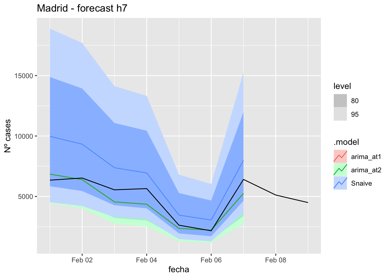
fc_h7 %>%
autoplot(
data_madrid %>%
filter(fecha <= as.Date("2022-01-31", format = "%Y-%m-%d")+days(9) &
fecha > as.Date("2021-12-01", format = "%Y-%m-%d"))
) +
labs(y = "Nº cases", title = "Madrid - forecast h7")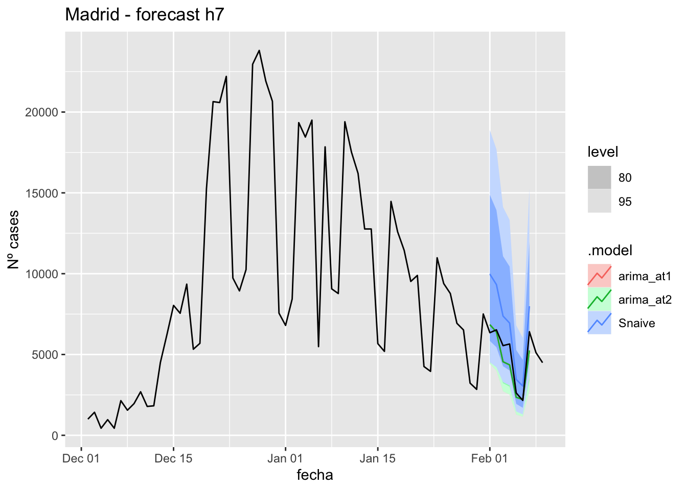
# Accuracy
fabletools::accuracy(fc_h7, data_madrid)# A tibble: 3 × 11
.model provincia .type ME RMSE MAE MPE MAPE MASE RMSSE ACF1
<chr> <chr> <chr> <dbl> <dbl> <dbl> <dbl> <dbl> <dbl> <dbl> <dbl>
1 arima_at1 Madrid Test 471. 788. 629. 8.70 11.7 0.843 0.441 0.0572
2 arima_at2 Madrid Test 471. 788. 629. 8.70 11.7 0.843 0.441 0.0572
3 Snaive Madrid Test -1836. 2070. 1836. -36.2 36.2 2.46 1.16 0.541 14 days
# Plots
fc_h14 %>%
autoplot(
data_madrid_test %>%
filter(fecha <= as.Date("2022-01-31", format = "%Y-%m-%d")+days(16))
) +
labs(y = "Nº cases", title = "Madrid - forecast h14")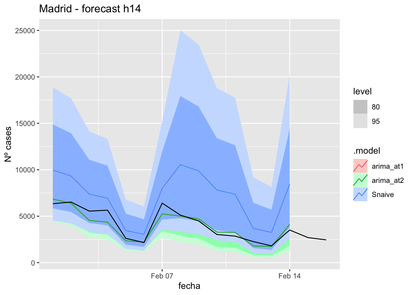
fc_h14 %>%
autoplot(
data_madrid %>%
filter(fecha <= as.Date("2022-01-31", format = "%Y-%m-%d")+days(16) &
fecha > as.Date("2021-12-01", format = "%Y-%m-%d"))
) +
labs(y = "Nº cases", title = "Madrid - forecast h14")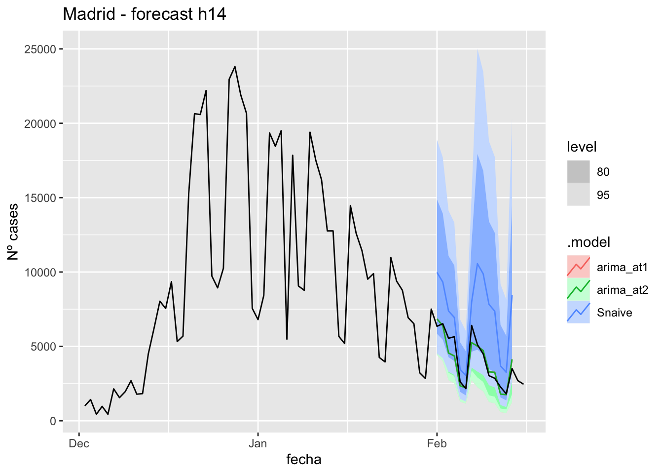
# Accuracy
fabletools::accuracy(fc_h14, data_madrid)# A tibble: 3 × 11
.model provincia .type ME RMSE MAE MPE MAPE MASE RMSSE ACF1
<chr> <chr> <chr> <dbl> <dbl> <dbl> <dbl> <dbl> <dbl> <dbl> <dbl>
1 arima_at1 Madrid Test 174. 612. 467. 2.98 10.9 0.625 0.343 0.215
2 arima_at2 Madrid Test 174. 612. 467. 2.98 10.9 0.625 0.343 0.215
3 Snaive Madrid Test -2914. 3386. 2914. -77.1 77.1 3.90 1.90 0.46621 days
# Plots
fc_h21 %>%
autoplot(
data_madrid_test %>%
filter(fecha <= as.Date("2022-01-31", format = "%Y-%m-%d")+days(23))
) +
labs(y = "Nº cases", title = "Madrid - forecast h21")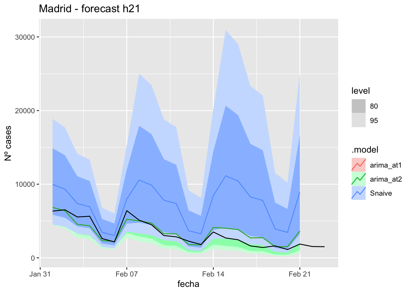
fc_h21 %>%
autoplot(
data_madrid %>%
filter(fecha <= as.Date("2022-01-31", format = "%Y-%m-%d")+days(23) &
fecha > as.Date("2021-12-01", format = "%Y-%m-%d"))
) +
labs(y = "Nº cases", title = "Madrid - forecast h21")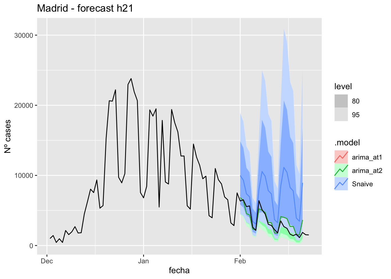
# Accuracy
fabletools::accuracy(fc_h21, data_madrid)# A tibble: 3 × 11
.model provincia .type ME RMSE MAE MPE MAPE MASE RMSSE ACF1
<chr> <chr> <chr> <dbl> <dbl> <dbl> <dbl> <dbl> <dbl> <dbl> <dbl>
1 arima_at1 Madrid Test -228. 851. 664. -16.7 26.5 0.888 0.477 0.512
2 arima_at2 Madrid Test -228. 851. 664. -16.7 26.5 0.888 0.477 0.512
3 Snaive Madrid Test -3903. 4584. 3903. -158. 158. 5.23 2.57 0.57457 days
# Plots
fc_h90 %>%
autoplot(
data_madrid_test %>%
filter(fecha <= as.Date("2022-01-31", format = "%Y-%m-%d")+days(59))
) +
labs(y = "Nº cases", title = "Madrid - forecast h90")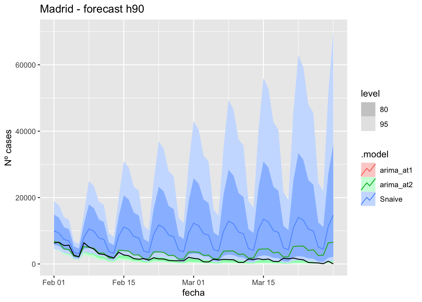
fc_h90 %>%
autoplot(
data_madrid %>%
filter(fecha <= as.Date("2022-01-31", format = "%Y-%m-%d")+days(59) &
fecha > as.Date("2021-12-01", format = "%Y-%m-%d"))
) +
labs(y = "Nº cases", title = "Madrid - forecast h90")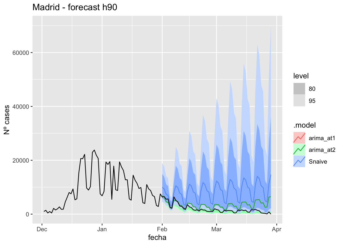
# Accuracy
fabletools::accuracy(fc_h90, data_madrid)# A tibble: 3 × 11
.model provincia .type ME RMSE MAE MPE MAPE MASE RMSSE ACF1
<chr> <chr> <chr> <dbl> <dbl> <dbl> <dbl> <dbl> <dbl> <dbl> <dbl>
1 arima_at1 Madrid Test -1540. 2217. 1701. -2124. 2127. 2.28 1.24 0.699
2 arima_at2 Madrid Test -1540. 2217. 1701. -2124. 2127. 2.28 1.24 0.699
3 Snaive Madrid Test -6507. 7446. 6507. -4965. 4965. 8.71 4.17 0.627Málaga
data_malaga <- covid_data %>%
filter(provincia == "Málaga") %>%
filter(fecha > as.Date("2020-06-14", format = "%Y-%m-%d")) %>%
select(provincia, fecha, num_casos, num_hosp, tmed,mob_grocery_pharmacy, mob_parks,
mob_residential, mob_retail_recreation, mob_transit_stations, mob_workplaces, mob_flujo) %>%
drop_na(-mob_flujo) %>%
as_tsibble(key = provincia, index = fecha)
data_malaga# A tsibble: 653 x 12 [1D]
# Key: provincia [1]
provincia fecha num_casos num_hosp tmed mob_grocery_pharmacy mob_parks
<chr> <date> <dbl> <dbl> <dbl> <dbl> <dbl>
1 Málaga 2020-06-15 1 0 27.2 -16 -9
2 Málaga 2020-06-16 1 0 27.8 -13 -4
3 Málaga 2020-06-17 2 0 26.9 -13 1
4 Málaga 2020-06-18 2 1 21.6 -12 3
5 Málaga 2020-06-19 1 0 24.7 -12 2
6 Málaga 2020-06-20 4 0 22.6 -14 8
7 Málaga 2020-06-21 4 0 22.7 -16 -3
8 Málaga 2020-06-22 6 0 25 -13 1
9 Málaga 2020-06-23 8 0 25.6 -10 18
10 Málaga 2020-06-24 65 2 24.5 -13 12
# … with 643 more rows, and 5 more variables: mob_residential <dbl>,
# mob_retail_recreation <dbl>, mob_transit_stations <dbl>,
# mob_workplaces <dbl>, mob_flujo <dbl>data_malaga_train <- data_malaga %>%
filter(fecha <= as.Date("2022-01-31", format = "%Y-%m-%d"))
summary(data_malaga_train$fecha) Min. 1st Qu. Median Mean 3rd Qu. Max.
"2020-06-15" "2020-11-10" "2021-04-08" "2021-04-08" "2021-09-04" "2022-01-31" data_malaga_test <- data_malaga %>%
filter(fecha > as.Date("2022-01-31", format = "%Y-%m-%d"))
summary(data_malaga_test$fecha) Min. 1st Qu. Median Mean 3rd Qu. Max.
"2022-02-01" "2022-02-15" "2022-03-01" "2022-03-01" "2022-03-15" "2022-03-29" lambda_Malaga <- data_malaga %>%
features(num_casos, features = guerrero) %>%
pull(lambda_guerrero)
fit_model <- data_malaga_train %>%
model(
arima_at1 = ARIMA(box_cox(num_casos, lambda_Malaga)),
arima_at2 = ARIMA(box_cox(num_casos, lambda_Malaga),
stepwise = FALSE, approx = FALSE),
Snaive = SNAIVE(box_cox(num_casos, lambda_Malaga))
)
# Show and report model
fit_model# A mable: 1 x 4
# Key: provincia [1]
provincia arima_at1 arima_at2 Snaive
<chr> <model> <model> <model>
1 Málaga <ARIMA(2,0,3)(0,1,1)[7]> <ARIMA(2,0,3)(0,1,1)[7]> <SNAIVE>glance(fit_model)# A tibble: 3 × 9
provincia .model sigma2 log_lik AIC AICc BIC ar_roots ma_roots
<chr> <chr> <dbl> <dbl> <dbl> <dbl> <dbl> <list> <list>
1 Málaga arima_at1 0.584 -679. 1372. 1372. 1402. <cpl [2]> <cpl [10]>
2 Málaga arima_at2 0.584 -679. 1372. 1372. 1402. <cpl [2]> <cpl [10]>
3 Málaga Snaive 2.41 NA NA NA NA <NULL> <NULL> fit_model %>%
pivot_longer(-provincia,
names_to = ".model",
values_to = "orders") %>%
left_join(glance(fit_model), by = c("provincia", ".model")) %>%
arrange(AICc) %>%
select(.model:BIC)# A mable: 3 x 7
# Key: .model [3]
.model orders sigma2 log_lik AIC AICc BIC
<chr> <model> <dbl> <dbl> <dbl> <dbl> <dbl>
1 arima_at1 <ARIMA(2,0,3)(0,1,1)[7]> 0.584 -679. 1372. 1372. 1402.
2 arima_at2 <ARIMA(2,0,3)(0,1,1)[7]> 0.584 -679. 1372. 1372. 1402.
3 Snaive <SNAIVE> 2.41 NA NA NA NA # We use a Ljung-Box test >> large p-value, confirms residuals are similar / considered to white noise
fit_model %>%
select(Snaive) %>%
gg_tsresiduals()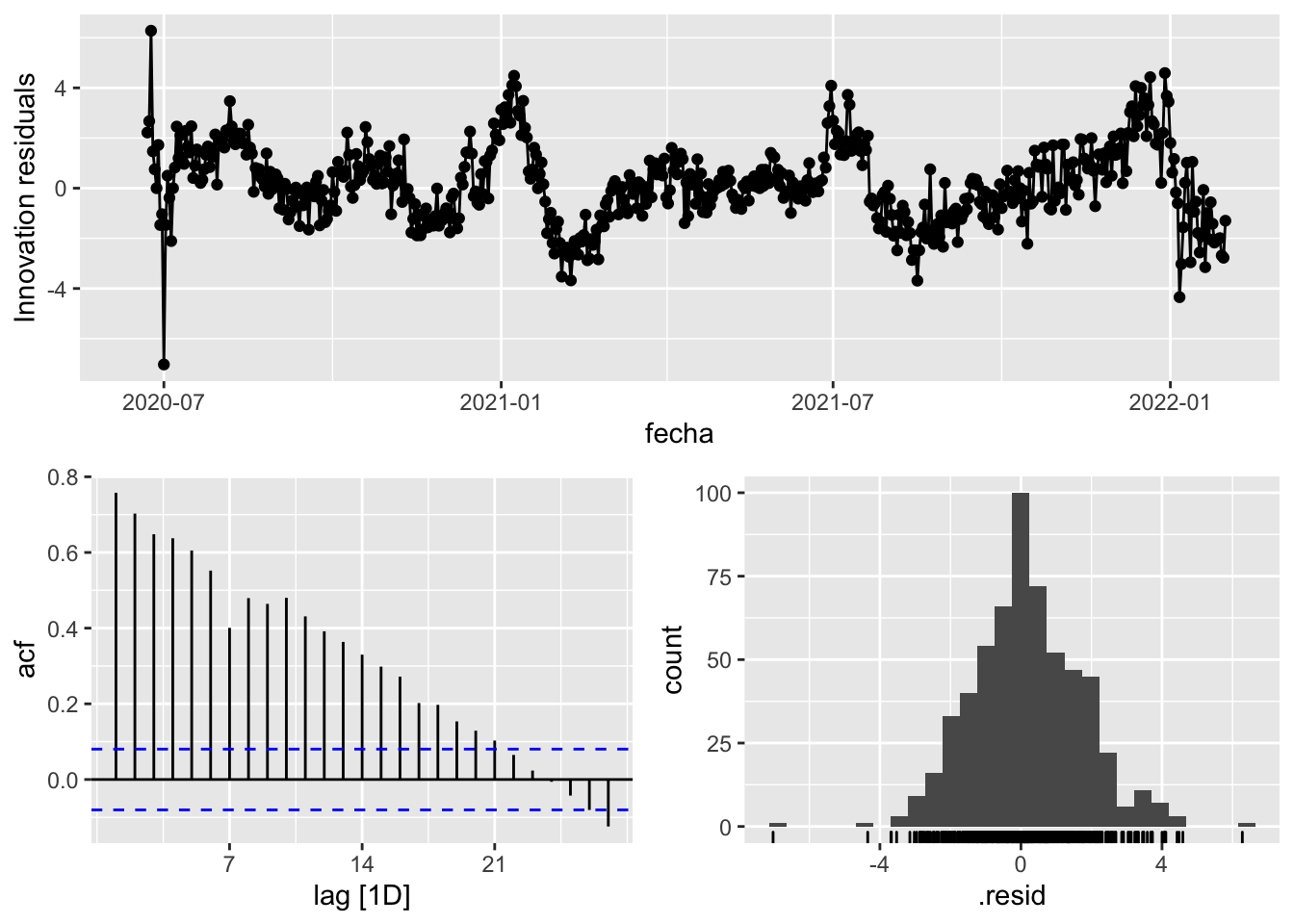
fit_model %>%
select(arima_at1) %>%
gg_tsresiduals()
fit_model %>%
select(arima_at2) %>%
gg_tsresiduals()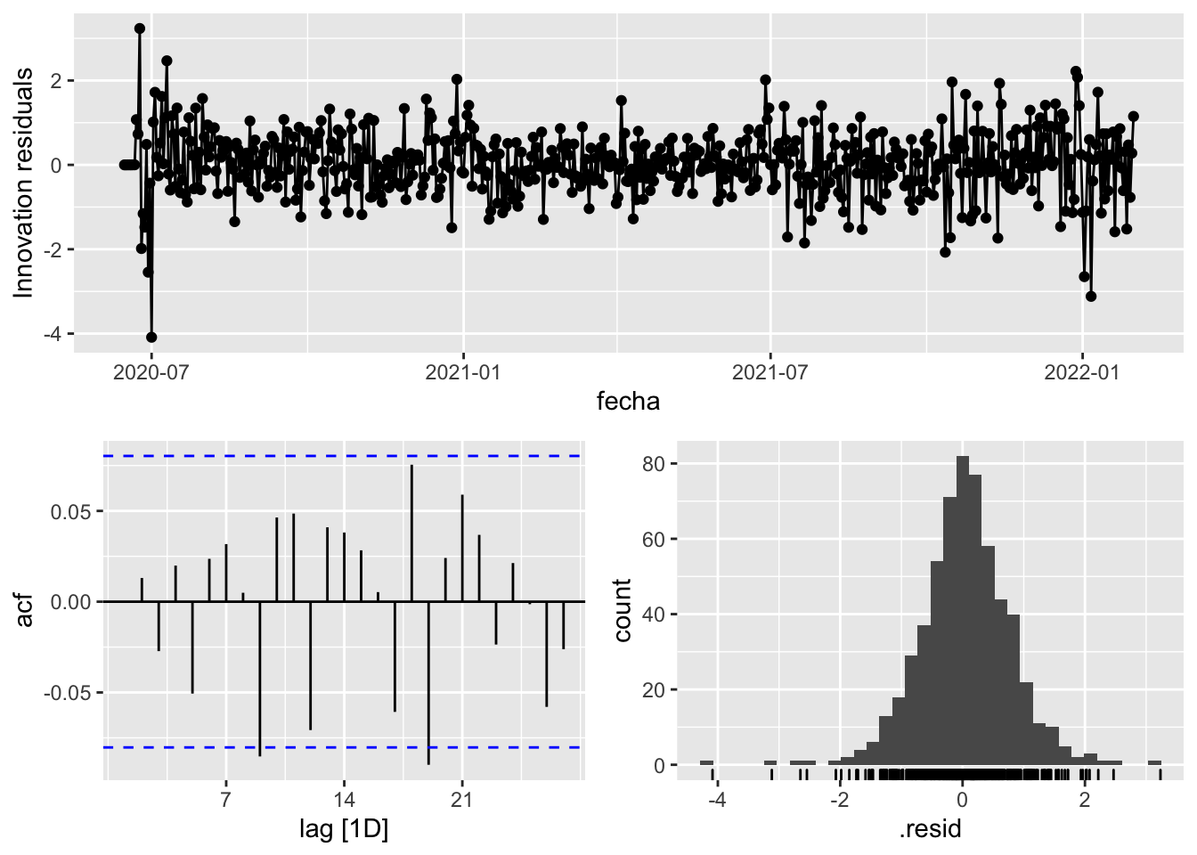
augment(fit_model) %>%
features(.innov, ljung_box, lag=7)# A tibble: 3 × 4
provincia .model lb_stat lb_pvalue
<chr> <chr> <dbl> <dbl>
1 Málaga arima_at1 3.28 0.858
2 Málaga arima_at2 3.28 0.858
3 Málaga Snaive 1621. 0 augment(fit_model) %>%
features(.innov, ljung_box, lag=14)# A tibble: 3 × 4
provincia .model lb_stat lb_pvalue
<chr> <chr> <dbl> <dbl>
1 Málaga arima_at1 15.4 0.350
2 Málaga arima_at2 15.4 0.350
3 Málaga Snaive 2376. 0 augment(fit_model) %>%
features(.innov, ljung_box, lag=21)# A tibble: 3 × 4
provincia .model lb_stat lb_pvalue
<chr> <chr> <dbl> <dbl>
1 Málaga arima_at1 29.2 0.109
2 Málaga arima_at2 29.2 0.109
3 Málaga Snaive 2555. 0 augment(fit_model) %>%
features(.innov, ljung_box, lag=57)# A tibble: 3 × 4
provincia .model lb_stat lb_pvalue
<chr> <chr> <dbl> <dbl>
1 Málaga arima_at1 58.4 0.423
2 Málaga arima_at2 58.4 0.423
3 Málaga Snaive 3422. 0 # Significant spikes out of 30 is still consistent with white noise
# To be sure, use a Ljung-Box test, which has a large p-value, confirming that
# the residuals are similar to white noise.
# Note that the alternative models also passed this test.
#
# Forecast
fc_h7 <- fabletools::forecast(fit_model, h = 7)
fc_h14 <- fabletools::forecast(fit_model, h = 14)
fc_h21 <- fabletools::forecast(fit_model, h = 21)
fc_h90 <- fabletools::forecast(fit_model, h = 57)7 days
# Plots
fc_h7 %>%
autoplot(
data_malaga_test %>%
filter(fecha <= as.Date("2022-01-31", format = "%Y-%m-%d")+days(9))
) +
labs(y = "Nº cases", title = "Malaga - forecast h7")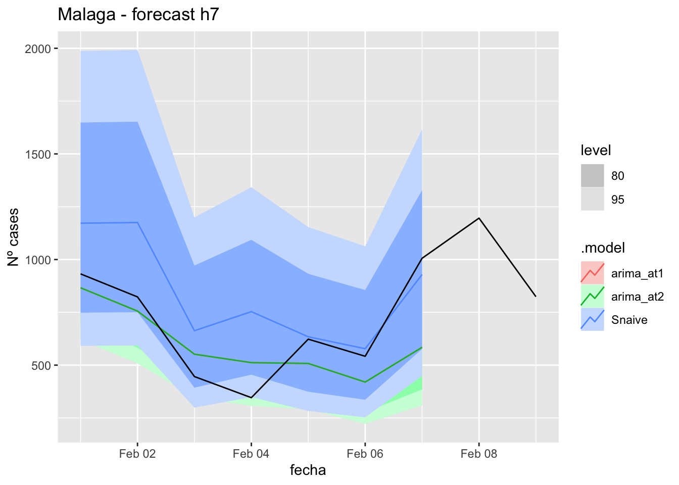
fc_h7 %>%
autoplot(
data_malaga %>%
filter(fecha <= as.Date("2022-01-31", format = "%Y-%m-%d")+days(9) &
fecha > as.Date("2021-12-01", format = "%Y-%m-%d"))
) +
labs(y = "Nº cases", title = "Malaga - forecast h7")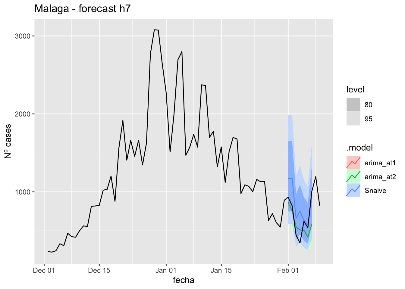
# Accuracy
fabletools::accuracy(fc_h7, data_malaga)# A tibble: 3 × 11
.model provincia .type ME RMSE MAE MPE MAPE MASE RMSSE ACF1
<chr> <chr> <chr> <dbl> <dbl> <dbl> <dbl> <dbl> <dbl> <dbl> <dbl>
1 arima_at1 Málaga Test 74.3 190. 152. 3.78 24.3 1.15 0.769 0.249
2 arima_at2 Málaga Test 74.3 190. 152. 3.78 24.3 1.15 0.769 0.249
3 Snaive Málaga Test -170. 240. 191. -33.7 35.9 1.45 0.968 0.24614 days
# Plots
fc_h14 %>%
autoplot(
data_malaga_test %>%
filter(fecha <= as.Date("2022-01-31", format = "%Y-%m-%d")+days(16))
) +
labs(y = "Nº cases", title = "Malaga - forecast h14")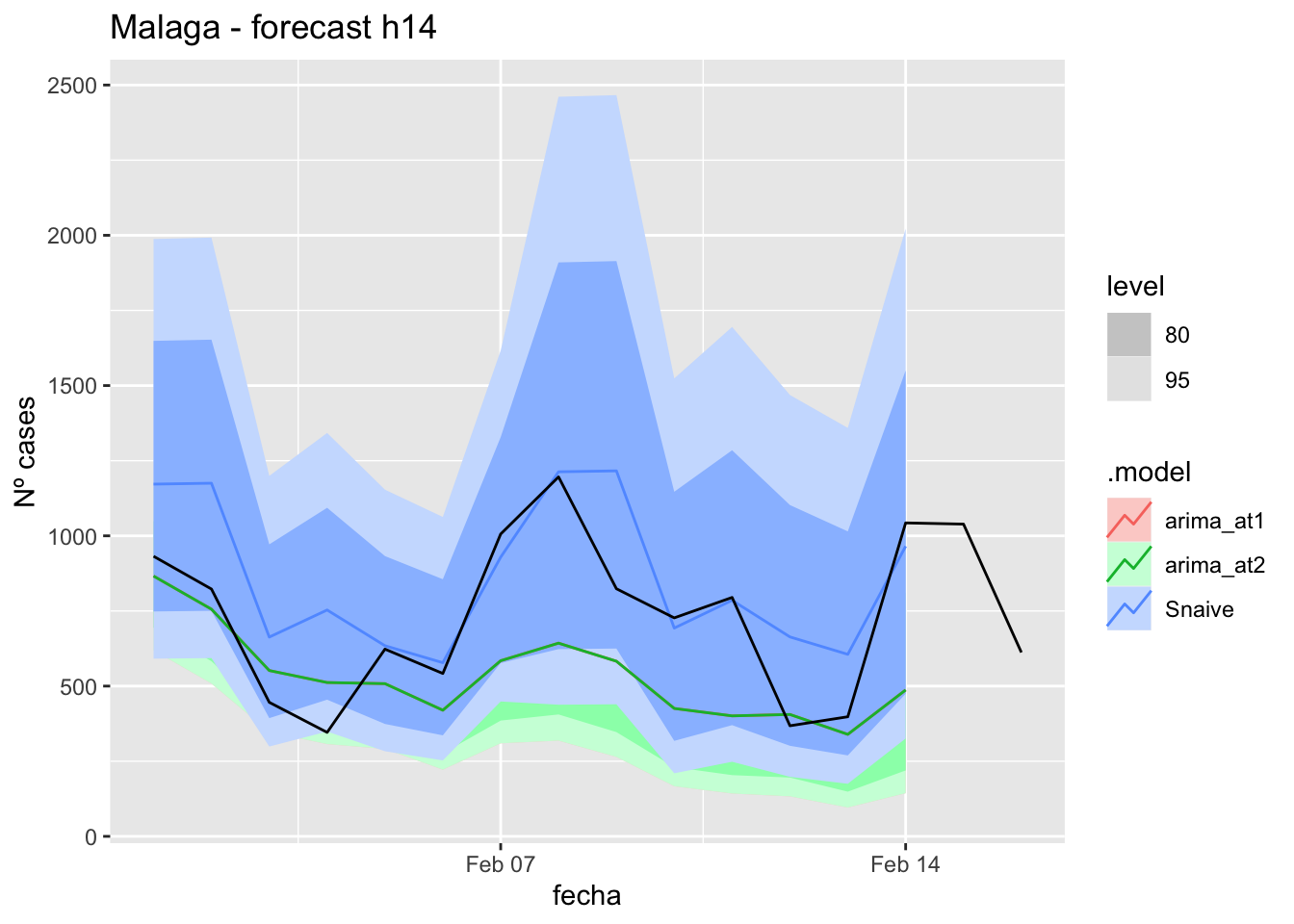
fc_h14 %>%
autoplot(
data_malaga %>%
filter(fecha <= as.Date("2022-01-31", format = "%Y-%m-%d")+days(16) &
fecha > as.Date("2021-12-01", format = "%Y-%m-%d"))
) +
labs(y = "Nº cases", title = "Malaga - forecast h14")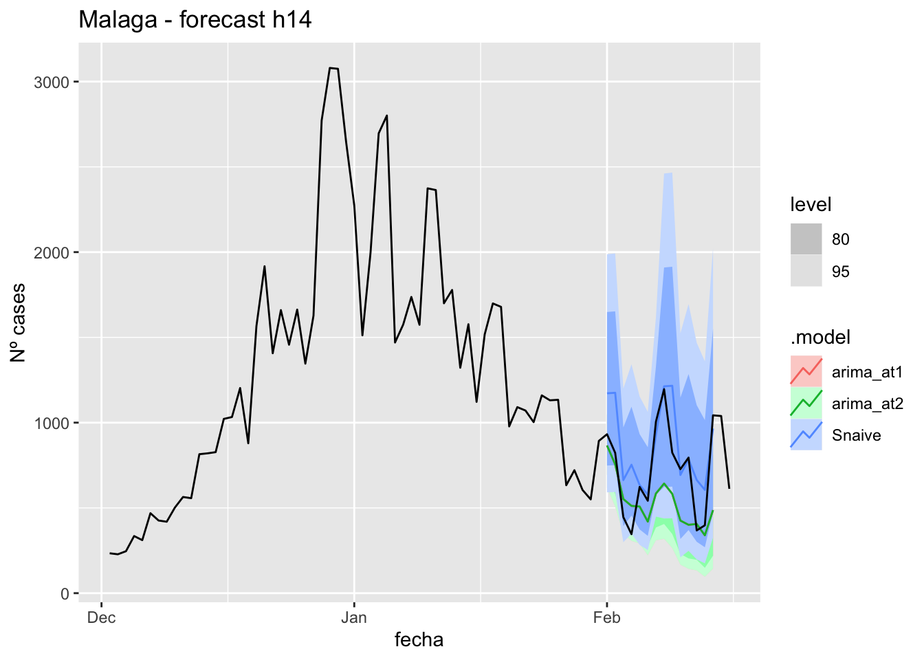
# Accuracy
fabletools::accuracy(fc_h14, data_malaga)# A tibble: 3 × 11
.model provincia .type ME RMSE MAE MPE MAPE MASE RMSSE ACF1
<chr> <chr> <chr> <dbl> <dbl> <dbl> <dbl> <dbl> <dbl> <dbl> <dbl>
1 arima_at1 Málaga Test 185. 290. 229. 17.9 29.6 1.73 1.17 0.340
2 arima_at2 Málaga Test 185. 290. 229. 17.9 29.6 1.73 1.17 0.340
3 Snaive Málaga Test -141. 223. 170. -28.9 31.8 1.28 0.899 0.023921 days
# Plots
fc_h21 %>%
autoplot(
data_malaga_test %>%
filter(fecha <= as.Date("2022-01-31", format = "%Y-%m-%d")+days(23))
) +
labs(y = "Nº cases", title = "Malaga - forecast h21")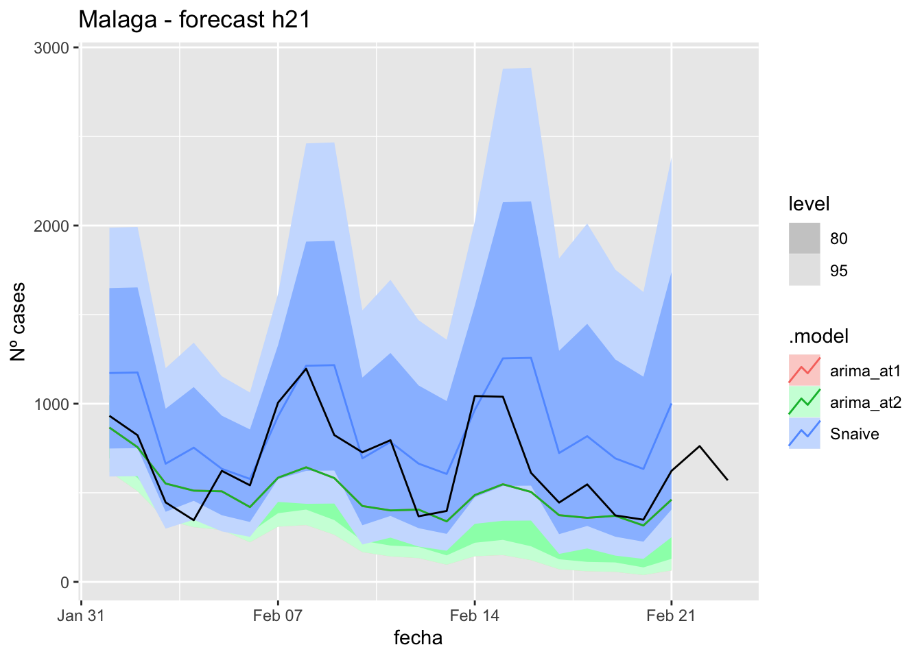
fc_h21 %>%
autoplot(
data_malaga %>%
filter(fecha <= as.Date("2022-01-31", format = "%Y-%m-%d")+days(23) &
fecha > as.Date("2021-12-01", format = "%Y-%m-%d"))
) +
labs(y = "Nº cases", title = "Malaga - forecast h21")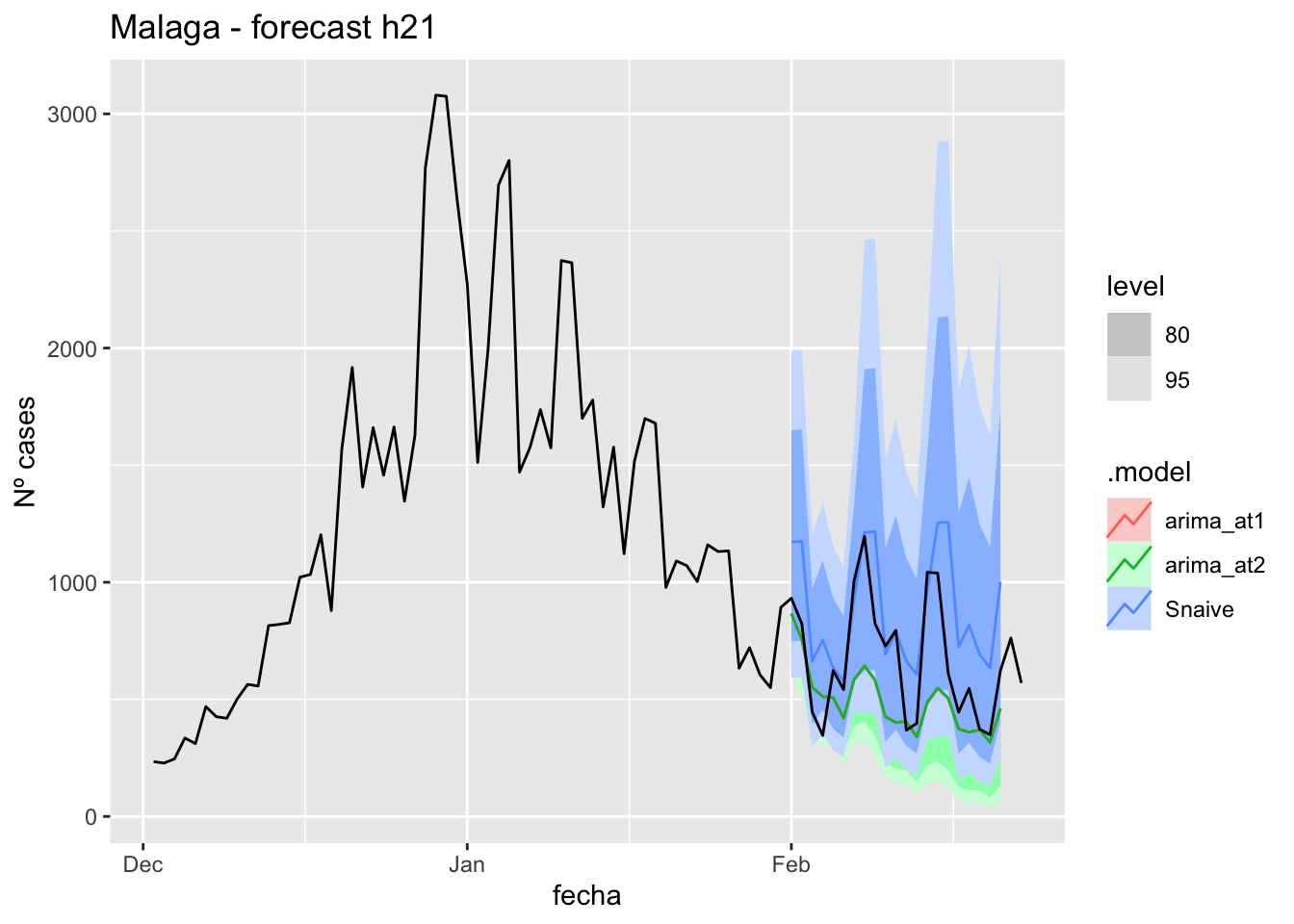
# Accuracy
fabletools::accuracy(fc_h21, data_malaga)# A tibble: 3 × 11
.model provincia .type ME RMSE MAE MPE MAPE MASE RMSSE ACF1
<chr> <chr> <chr> <dbl> <dbl> <dbl> <dbl> <dbl> <dbl> <dbl> <dbl>
1 arima_at1 Málaga Test 173. 267. 203. 19.1 26.9 1.53 1.08 0.422
2 arima_at2 Málaga Test 173. 267. 203. 19.1 26.9 1.53 1.08 0.422
3 Snaive Málaga Test -208. 279. 227. -41.4 43.4 1.72 1.13 0.17257 days
# Plots
fc_h90 %>%
autoplot(
data_malaga_test %>%
filter(fecha <= as.Date("2022-01-31", format = "%Y-%m-%d")+days(59))
) +
labs(y = "Nº cases", title = "Malaga - forecast h90")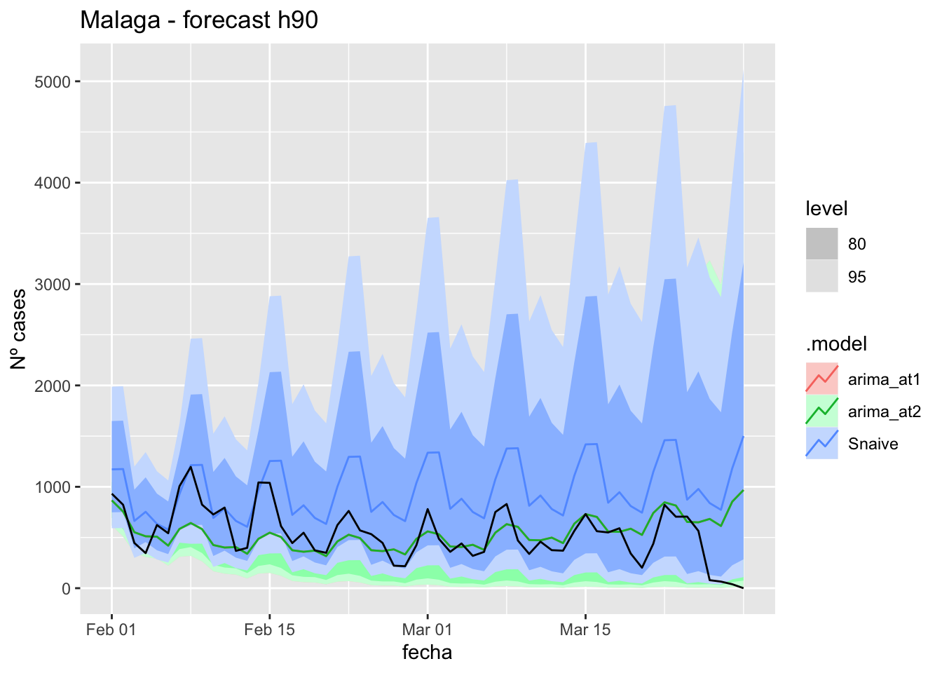
fc_h90 %>%
autoplot(
data_malaga %>%
filter(fecha <= as.Date("2022-01-31", format = "%Y-%m-%d")+days(59) &
fecha > as.Date("2021-12-01", format = "%Y-%m-%d"))
) +
labs(y = "Nº cases", title = "Malaga - forecast h90")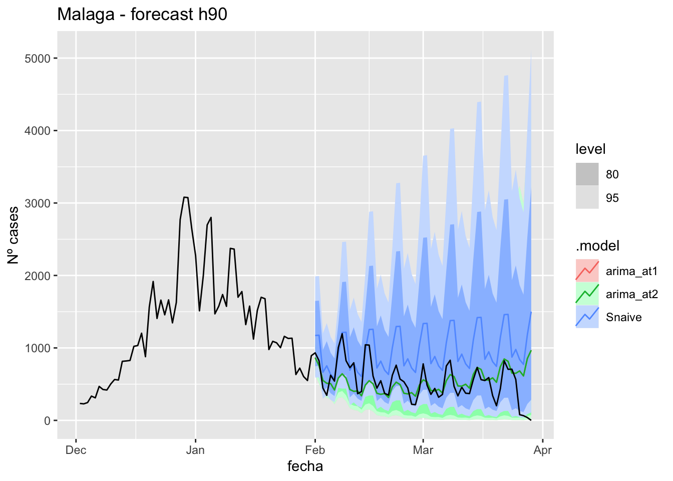
# Accuracy
fabletools::accuracy(fc_h90, data_malaga)# A tibble: 3 × 11
.model provincia .type ME RMSE MAE MPE MAPE MASE RMSSE ACF1
<chr> <chr> <chr> <dbl> <dbl> <dbl> <dbl> <dbl> <dbl> <dbl> <dbl>
1 arima_at1 Málaga Test -6.39 278. 190. -Inf Inf 1.44 1.12 0.656
2 arima_at2 Málaga Test -6.39 278. 190. -Inf Inf 1.44 1.12 0.656
3 Snaive Málaga Test -436. 525. 443. -Inf Inf 3.35 2.12 0.513Sevilla
data_sevilla <- covid_data %>%
filter(provincia == "Sevilla") %>%
filter(fecha > as.Date("2020-06-14", format = "%Y-%m-%d")) %>%
select(provincia, fecha, num_casos, num_hosp, tmed,mob_grocery_pharmacy, mob_parks,
mob_residential, mob_retail_recreation, mob_transit_stations, mob_workplaces, mob_flujo) %>%
drop_na(-mob_flujo) %>%
as_tsibble(key = provincia, index = fecha)
data_sevilla# A tsibble: 653 x 12 [1D]
# Key: provincia [1]
provincia fecha num_casos num_hosp tmed mob_grocery_pharmacy mob_parks
<chr> <date> <dbl> <dbl> <dbl> <dbl> <dbl>
1 Sevilla 2020-06-15 2 1 23.1 -14 -13
2 Sevilla 2020-06-16 1 0 24.0 -10 -4
3 Sevilla 2020-06-17 0 0 24.9 -10 -7
4 Sevilla 2020-06-18 0 0 25.8 -12 -13
5 Sevilla 2020-06-19 0 0 26.6 -13 -20
6 Sevilla 2020-06-20 0 0 27.5 -20 -34
7 Sevilla 2020-06-21 0 0 28.4 -27 -47
8 Sevilla 2020-06-22 1 0 29.3 -17 -19
9 Sevilla 2020-06-23 0 0 30.2 -12 -13
10 Sevilla 2020-06-24 1 0 29.4 -12 -12
# … with 643 more rows, and 5 more variables: mob_residential <dbl>,
# mob_retail_recreation <dbl>, mob_transit_stations <dbl>,
# mob_workplaces <dbl>, mob_flujo <dbl>data_sevilla_train <- data_sevilla %>%
filter(fecha <= as.Date("2022-01-31", format = "%Y-%m-%d"))
summary(data_sevilla_train$fecha) Min. 1st Qu. Median Mean 3rd Qu. Max.
"2020-06-15" "2020-11-10" "2021-04-08" "2021-04-08" "2021-09-04" "2022-01-31" data_sevilla_test <- data_sevilla %>%
filter(fecha > as.Date("2022-01-31", format = "%Y-%m-%d"))
summary(data_sevilla_test$fecha) Min. 1st Qu. Median Mean 3rd Qu. Max.
"2022-02-01" "2022-02-15" "2022-03-01" "2022-03-01" "2022-03-15" "2022-03-29" lambda_Sevilla <- data_sevilla %>%
features(num_casos, features = guerrero) %>%
pull(lambda_guerrero)
fit_model <- data_sevilla_train %>%
model(
arima_at1 = ARIMA(box_cox(num_casos, lambda_Sevilla)),
arima_at2 = ARIMA(box_cox(num_casos, lambda_Sevilla),
stepwise = FALSE, approx = FALSE),
Snaive = SNAIVE(box_cox(num_casos, lambda_Sevilla))
)
# Show and report model
fit_model# A mable: 1 x 4
# Key: provincia [1]
provincia arima_at1 arima_at2 Snaive
<chr> <model> <model> <model>
1 Sevilla <ARIMA(3,1,1)(2,0,0)[7]> <ARIMA(4,1,0)(2,0,0)[7]> <SNAIVE>glance(fit_model)# A tibble: 3 × 9
provincia .model sigma2 log_lik AIC AICc BIC ar_roots ma_roots
<chr> <chr> <dbl> <dbl> <dbl> <dbl> <dbl> <list> <list>
1 Sevilla arima_at1 0.962 -832. 1679. 1679. 1709. <cpl [17]> <cpl [1]>
2 Sevilla arima_at2 0.962 -832. 1678. 1679. 1709. <cpl [18]> <cpl [0]>
3 Sevilla Snaive 2.23 NA NA NA NA <NULL> <NULL> fit_model %>%
pivot_longer(-provincia,
names_to = ".model",
values_to = "orders") %>%
left_join(glance(fit_model), by = c("provincia", ".model")) %>%
arrange(AICc) %>%
select(.model:BIC)# A mable: 3 x 7
# Key: .model [3]
.model orders sigma2 log_lik AIC AICc BIC
<chr> <model> <dbl> <dbl> <dbl> <dbl> <dbl>
1 arima_at2 <ARIMA(4,1,0)(2,0,0)[7]> 0.962 -832. 1678. 1679. 1709.
2 arima_at1 <ARIMA(3,1,1)(2,0,0)[7]> 0.962 -832. 1679. 1679. 1709.
3 Snaive <SNAIVE> 2.23 NA NA NA NA # We use a Ljung-Box test >> large p-value, confirms residuals are similar / considered to white noise
fit_model %>%
select(Snaive) %>%
gg_tsresiduals()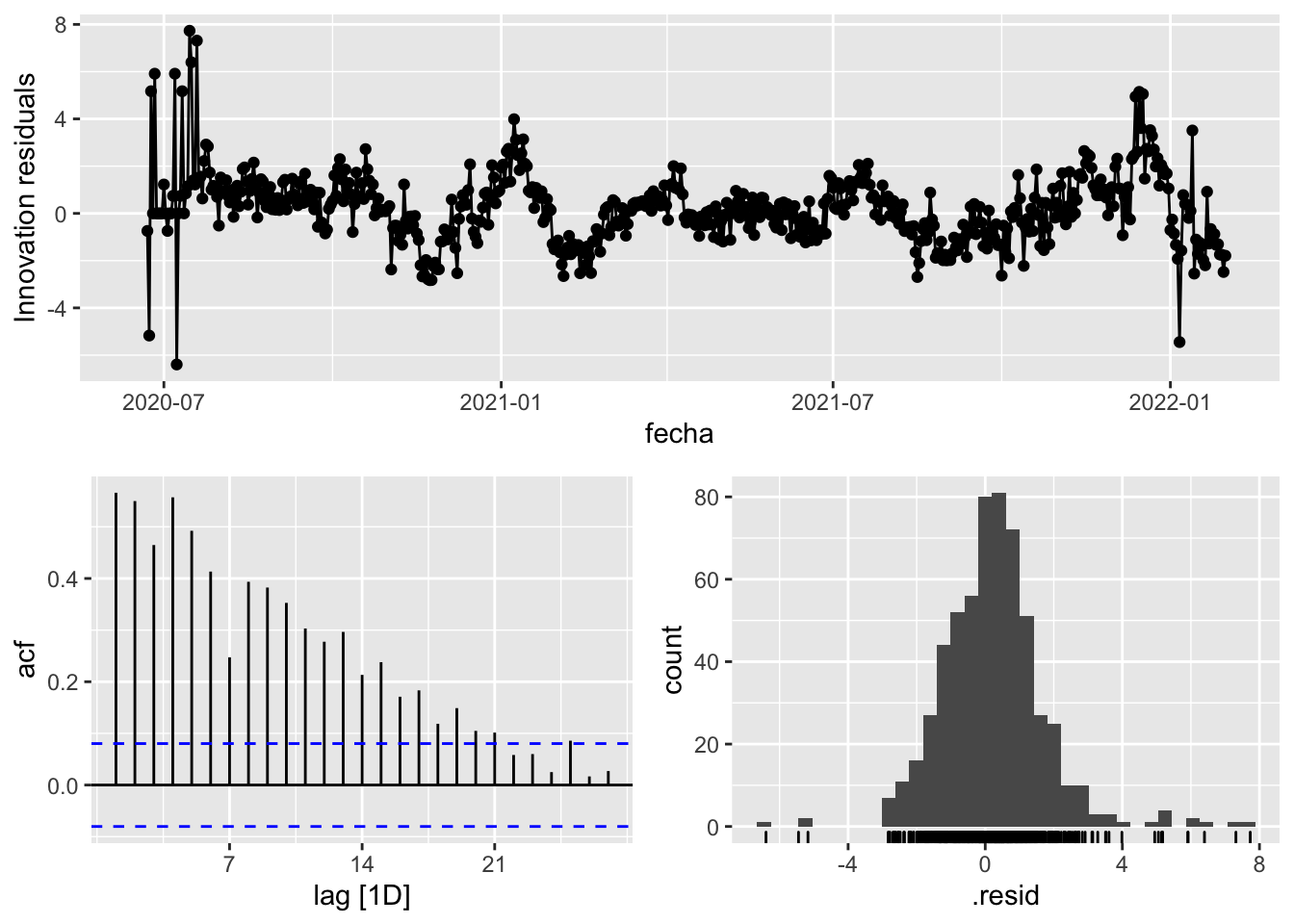
fit_model %>%
select(arima_at1) %>%
gg_tsresiduals()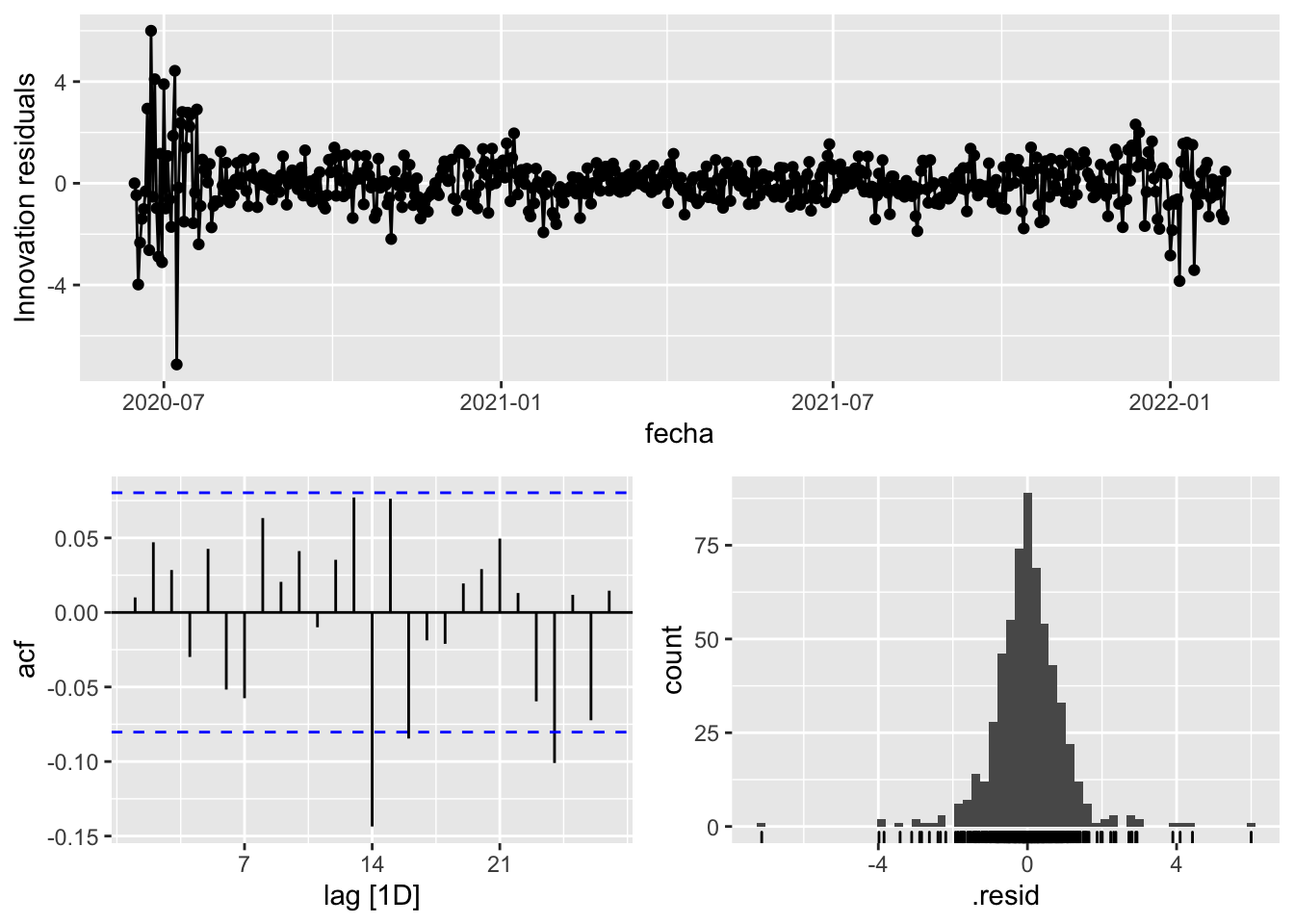
fit_model %>%
select(arima_at2) %>%
gg_tsresiduals()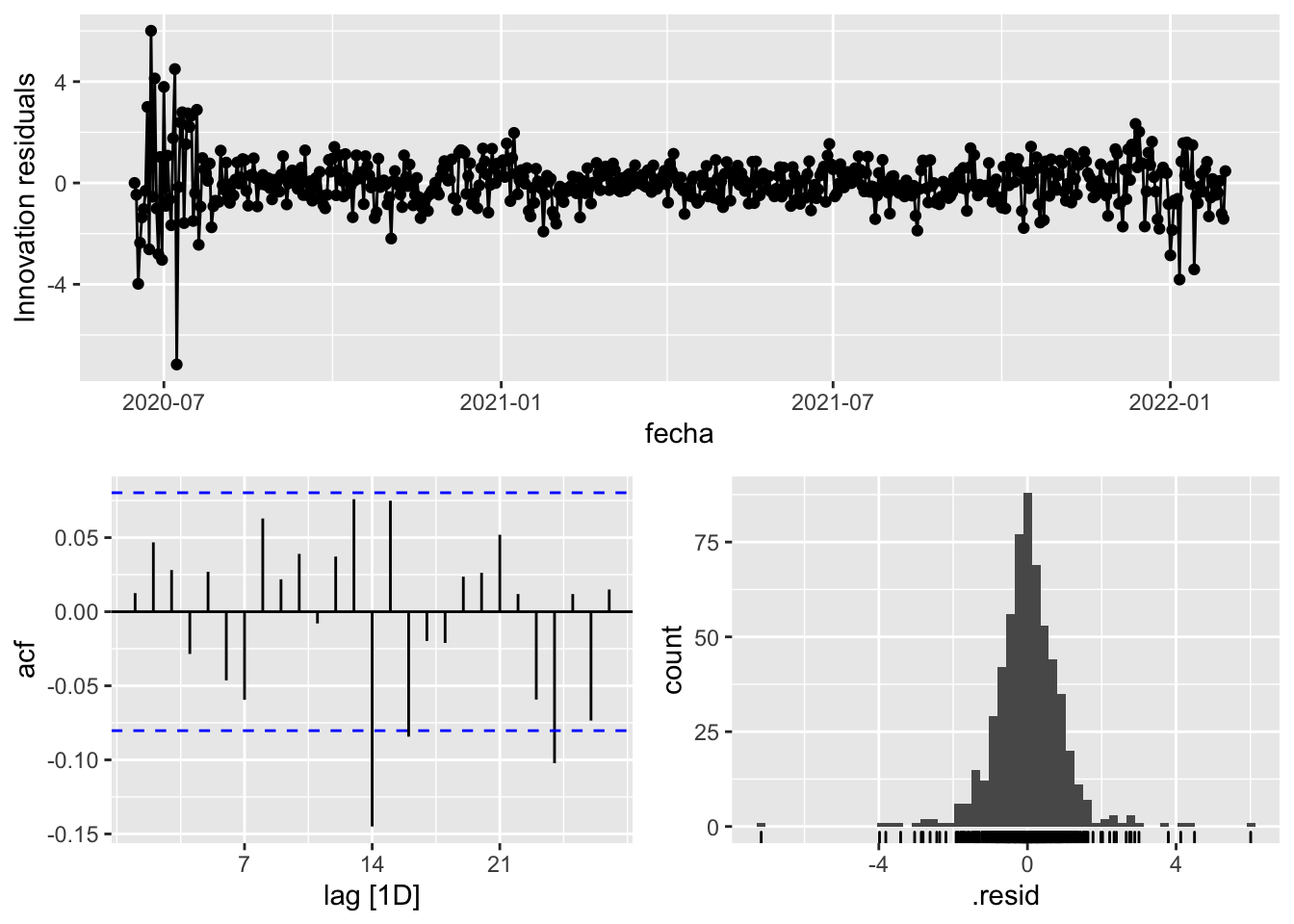
augment(fit_model) %>%
features(.innov, ljung_box, lag=7)# A tibble: 3 × 4
provincia .model lb_stat lb_pvalue
<chr> <chr> <dbl> <dbl>
1 Sevilla arima_at1 7.13 0.416
2 Sevilla arima_at2 6.24 0.512
3 Sevilla Snaive 965. 0 augment(fit_model) %>%
features(.innov, ljung_box, lag=14)# A tibble: 3 × 4
provincia .model lb_stat lb_pvalue
<chr> <chr> <dbl> <dbl>
1 Sevilla arima_at1 27.9 0.0146
2 Sevilla arima_at2 27.1 0.0185
3 Sevilla Snaive 1403. 0 augment(fit_model) %>%
features(.innov, ljung_box, lag=21)# A tibble: 3 × 4
provincia .model lb_stat lb_pvalue
<chr> <chr> <dbl> <dbl>
1 Sevilla arima_at1 38.6 0.0108
2 Sevilla arima_at2 37.9 0.0132
3 Sevilla Snaive 1510. 0 augment(fit_model) %>%
features(.innov, ljung_box, lag=57)# A tibble: 3 × 4
provincia .model lb_stat lb_pvalue
<chr> <chr> <dbl> <dbl>
1 Sevilla arima_at1 78.0 0.0335
2 Sevilla arima_at2 77.4 0.0372
3 Sevilla Snaive 1813. 0 # Significant spikes out of 30 is still consistent with white noise
# To be sure, use a Ljung-Box test, which has a large p-value, confirming that
# the residuals are similar to white noise.
# Note that the alternative models also passed this test.
#
# Forecast
fc_h7 <- fabletools::forecast(fit_model, h = 7)
fc_h14 <- fabletools::forecast(fit_model, h = 14)
fc_h21 <- fabletools::forecast(fit_model, h = 21)
fc_h90 <- fabletools::forecast(fit_model, h = 57)7 days
# Plots
fc_h7 %>%
autoplot(
data_sevilla_test %>%
filter(fecha <= as.Date("2022-01-31", format = "%Y-%m-%d")+days(9))
) +
labs(y = "Nº cases", title = "Sevilla - forecast h7")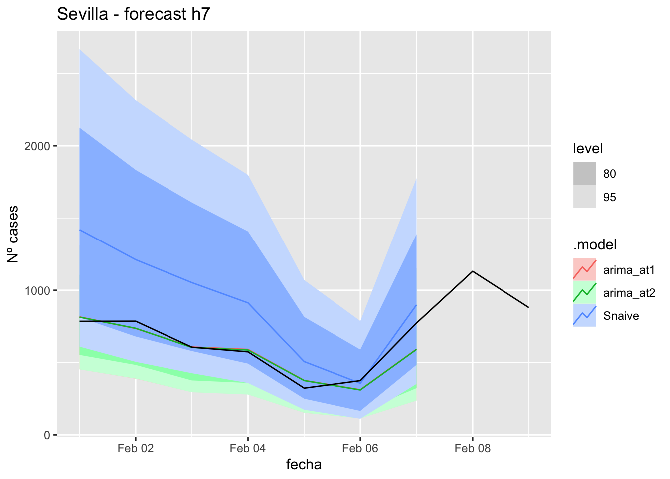
fc_h7 %>%
autoplot(
data_sevilla %>%
filter(fecha <= as.Date("2022-01-31", format = "%Y-%m-%d")+days(9) &
fecha > as.Date("2021-12-01", format = "%Y-%m-%d"))
) +
labs(y = "Nº cases", title = "Sevilla - forecast h7")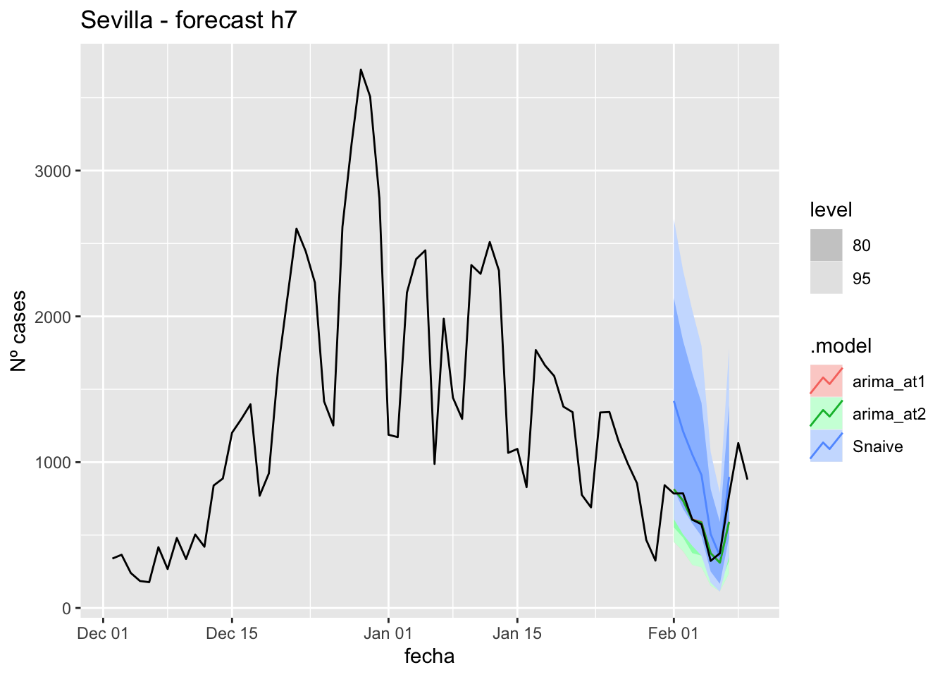
# Accuracy
fabletools::accuracy(fc_h7, data_sevilla)# A tibble: 3 × 11
.model provincia .type ME RMSE MAE MPE MAPE MASE RMSSE ACF1
<chr> <chr> <chr> <dbl> <dbl> <dbl> <dbl> <dbl> <dbl> <dbl> <dbl>
1 arima_at1 Sevilla Test 27.5 78.6 56.6 3.30 10.0 0.396 0.288 0.143
2 arima_at2 Sevilla Test 29.1 78.8 55.9 3.60 9.91 0.391 0.289 0.142
3 Snaive Sevilla Test -305. 368. 311. -48.0 49.4 2.17 1.35 0.52314 days
# Plots
fc_h14 %>%
autoplot(
data_sevilla_test %>%
filter(fecha <= as.Date("2022-01-31", format = "%Y-%m-%d")+days(16))
) +
labs(y = "Nº cases", title = "Sevilla - forecast h14")
fc_h14 %>%
autoplot(
data_sevilla %>%
filter(fecha <= as.Date("2022-01-31", format = "%Y-%m-%d")+days(16) &
fecha > as.Date("2021-12-01", format = "%Y-%m-%d"))
) +
labs(y = "Nº cases", title = "Sevilla - forecast h14")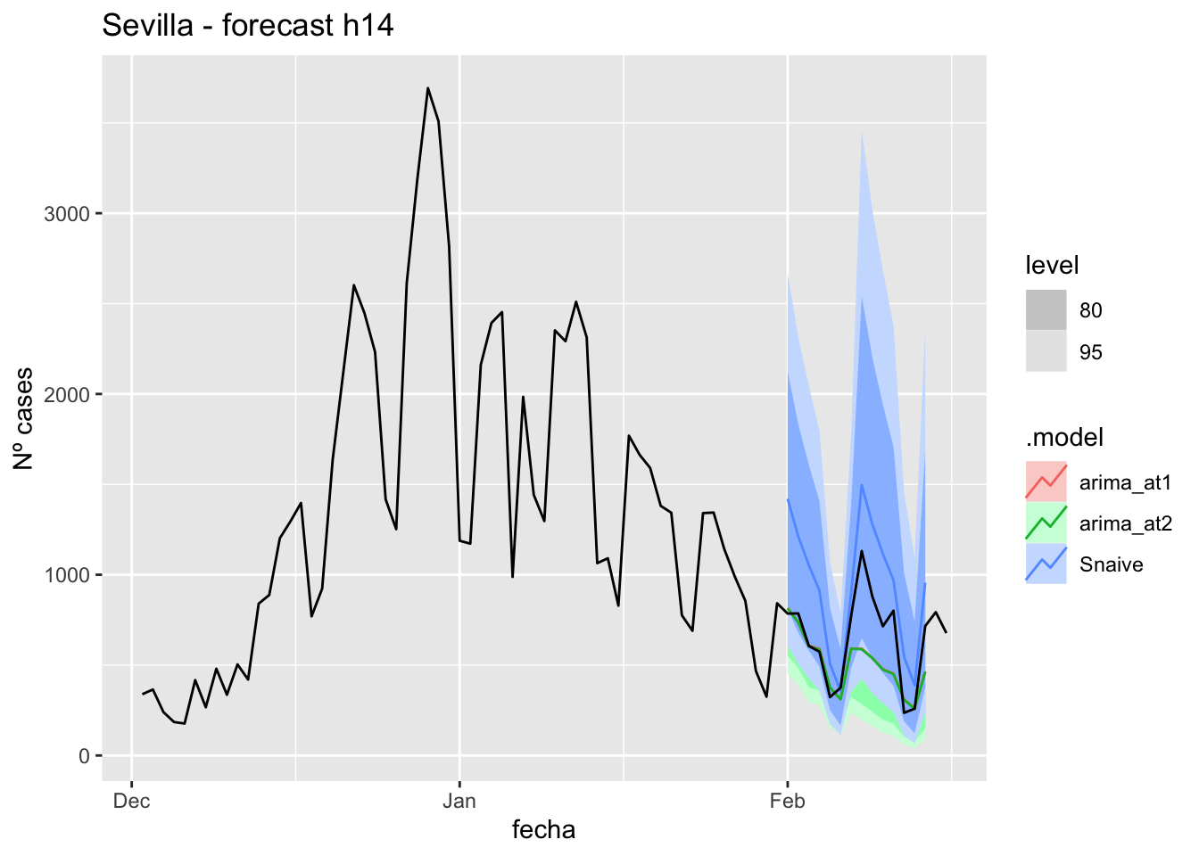
# Accuracy
fabletools::accuracy(fc_h14, data_sevilla)# A tibble: 3 × 11
.model provincia .type ME RMSE MAE MPE MAPE MASE RMSSE ACF1
<chr> <chr> <chr> <dbl> <dbl> <dbl> <dbl> <dbl> <dbl> <dbl> <dbl>
1 arima_at1 Sevilla Test 131. 223. 156. 13.5 21.5 1.09 0.817 0.433
2 arima_at2 Sevilla Test 133. 224. 157. 13.9 21.4 1.09 0.822 0.432
3 Snaive Sevilla Test -297. 338. 299. -50.4 51.1 2.09 1.24 0.41121 days
# Plots
fc_h21 %>%
autoplot(
data_sevilla_test %>%
filter(fecha <= as.Date("2022-01-31", format = "%Y-%m-%d")+days(23))
) +
labs(y = "Nº cases", title = "Sevilla - forecast h21")
fc_h21 %>%
autoplot(
data_sevilla %>%
filter(fecha <= as.Date("2022-01-31", format = "%Y-%m-%d")+days(23) &
fecha > as.Date("2021-12-01", format = "%Y-%m-%d"))
) +
labs(y = "Nº cases", title = "Sevilla - forecast h21")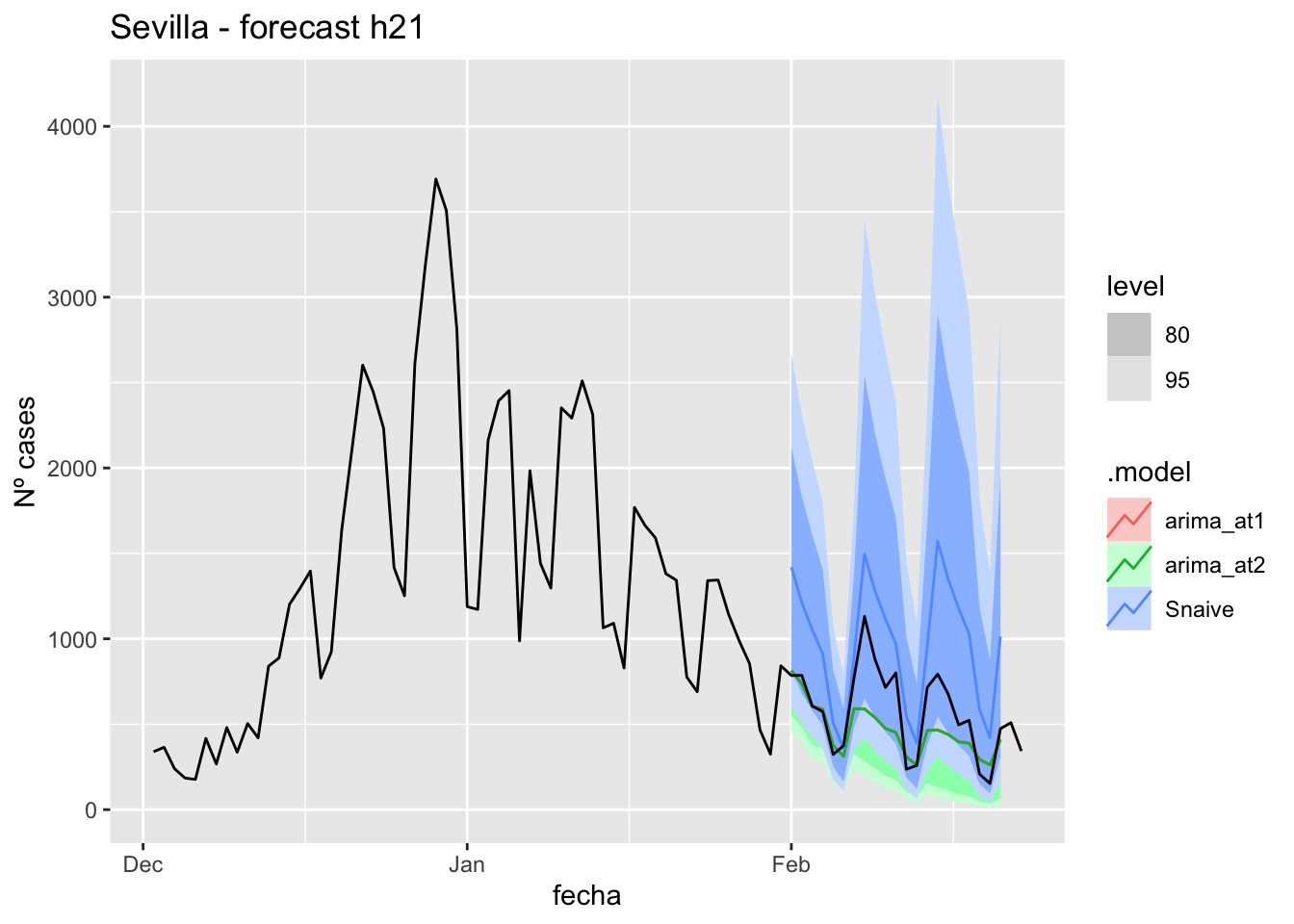
# Accuracy
fabletools::accuracy(fc_h21, data_sevilla)# A tibble: 3 × 11
.model provincia .type ME RMSE MAE MPE MAPE MASE RMSSE ACF1
<chr> <chr> <chr> <dbl> <dbl> <dbl> <dbl> <dbl> <dbl> <dbl> <dbl>
1 arima_at1 Sevilla Test 118. 208. 154. 9.96 26.1 1.08 0.762 0.499
2 arima_at2 Sevilla Test 121. 209. 155. 10.4 26.0 1.08 0.767 0.498
3 Snaive Sevilla Test -380. 430. 381. -76.5 77.0 2.67 1.58 0.50757 days
# Plots
fc_h90 %>%
autoplot(
data_sevilla_test %>%
filter(fecha <= as.Date("2022-01-31", format = "%Y-%m-%d")+days(59))
) +
labs(y = "Nº cases", title = "Sevilla - forecast h90")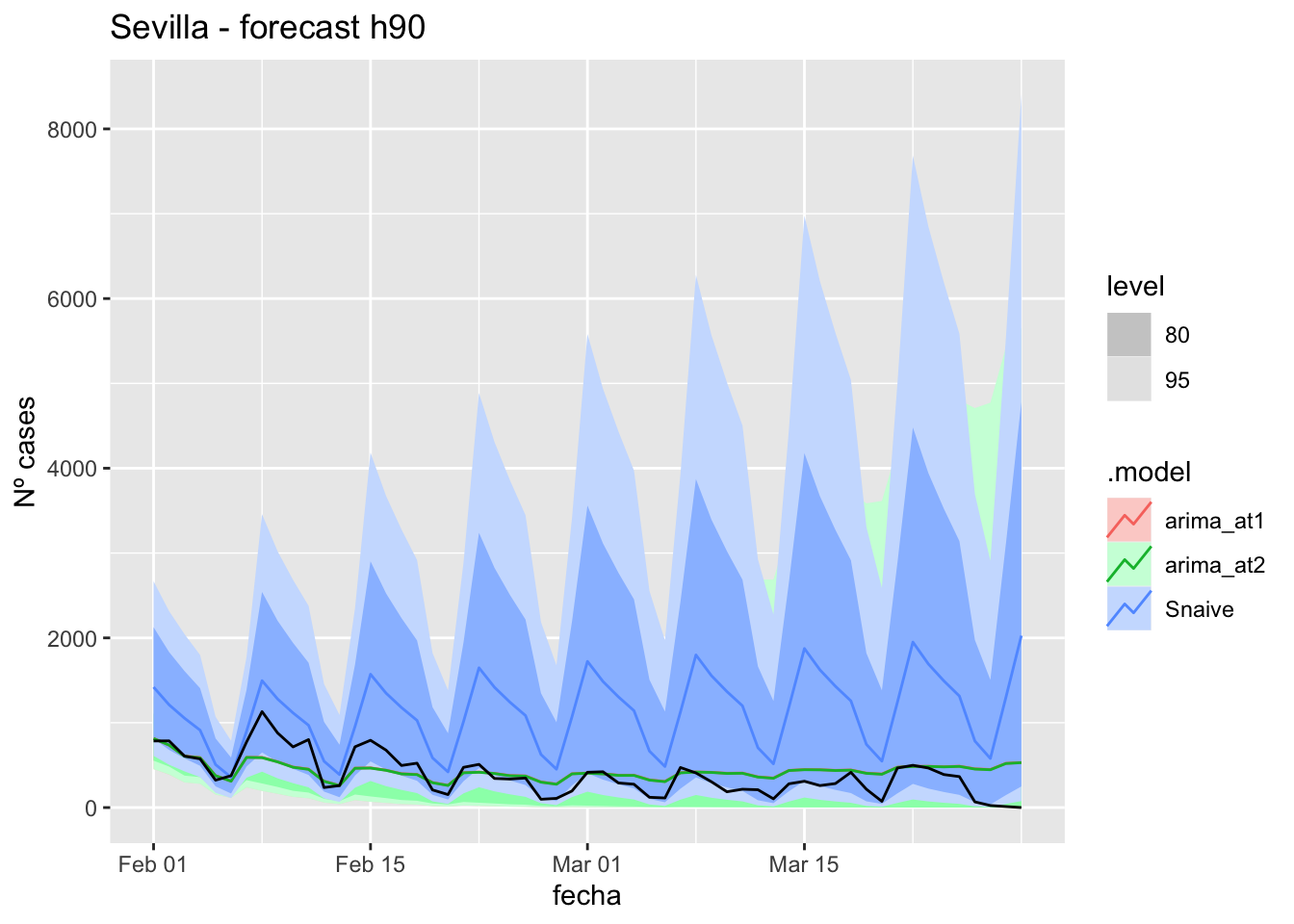
fc_h90 %>%
autoplot(
data_sevilla %>%
filter(fecha <= as.Date("2022-01-31", format = "%Y-%m-%d")+days(59) &
fecha > as.Date("2021-12-01", format = "%Y-%m-%d"))
) +
labs(y = "Nº cases", title = "Sevilla - forecast h90")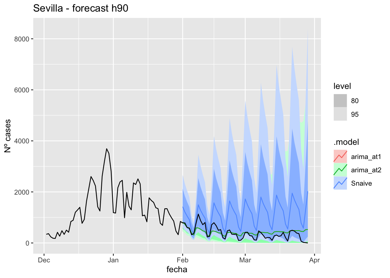
# Accuracy
fabletools::accuracy(fc_h90, data_sevilla)# A tibble: 3 × 11
.model provincia .type ME RMSE MAE MPE MAPE MASE RMSSE ACF1
<chr> <chr> <chr> <dbl> <dbl> <dbl> <dbl> <dbl> <dbl> <dbl> <dbl>
1 arima_at1 Sevilla Test -49.7 208. 157. -Inf Inf 1.10 0.761 0.718
2 arima_at2 Sevilla Test -47.4 207. 156. -Inf Inf 1.09 0.759 0.717
3 Snaive Sevilla Test -737. 850. 738. -Inf Inf 5.16 3.11 0.642