LSTM univariate prediction

Import python packages:

import numpy as np
import pandas as pd
import matplotlib
import matplotlib.pyplot as plt

from sklearn.preprocessing import MinMaxScaler
from sklearn.metrics import mean_absolute_error, mean_squared_error

from keras import Input
from keras.models import Sequential
from keras.layers import Dense, LSTM
from keras.layers.core import Dense, Activation, Dropout

data_covid = pd.read_csv('data/clean/final_covid_data.csv')
data_covid

	provincia	fecha	num_casos	num_casos_prueba_pcr	num_casos_prueba_test_ac	num_casos_prueba_ag	num_casos_prueba_elisa	num_casos_prueba_desconocida	num_hosp	num_uci	...	ws	ws_max	sol	mob_grocery_pharmacy	mob_parks	mob_residential	mob_retail_recreation	mob_transit_stations	mob_workplaces	mob_flujo
0	Barcelona	2020-01-01	0	0	0	0	0	0	0	0	...	2.5	7.2	4.9	NaN	NaN	NaN	NaN	NaN	NaN	NaN
1	Madrid	2020-01-01	1	1	0	0	0	0	1	0	...	0.8	3.6	8.3	NaN	NaN	NaN	NaN	NaN	NaN	NaN
2	Málaga	2020-01-01	0	0	0	0	0	0	0	0	...	3.3	6.7	7.7	NaN	NaN	NaN	NaN	NaN	NaN	NaN
3	Asturias	2020-01-01	0	0	0	0	0	0	0	0	...	2.5	7.8	7.9	NaN	NaN	NaN	NaN	NaN	NaN	NaN
4	Sevilla	2020-01-01	0	0	0	0	0	0	1	0	...	1.9	5.8	9.1	NaN	NaN	NaN	NaN	NaN	NaN	NaN
...	...	...	...	...	...	...	...	...	...	...	...	...	...	...	...	...	...	...	...	...	...
4090	Barcelona	2022-03-29	0	0	0	0	0	0	0	0	...	7.2	13.3	0.0	0.0	-13.0	5.0	-24.0	-16.0	-17.0	NaN
4091	Madrid	2022-03-29	6	3	0	3	0	0	0	0	...	2.2	6.1	2.4	1.0	-11.0	4.0	-25.0	-16.0	-16.0	NaN
4092	Málaga	2022-03-29	0	0	0	0	0	0	0	0	...	4.2	10.8	1.5	4.0	-3.0	4.0	-16.0	1.0	-8.0	NaN
4093	Asturias	2022-03-29	0	0	0	0	0	0	1	0	...	2.2	6.7	0.0	-4.0	17.0	3.0	-25.0	-15.0	-12.0	NaN
4094	Sevilla	2022-03-29	0	0	0	0	0	0	0	0	...	2.5	8.3	1.6	3.0	-7.0	2.0	-15.0	-13.0	-5.0	NaN

4095 rows × 26 columns

All the available data

We will only detele data from the first wave since it is not reliable.

Asturias

data_asturias = data_covid.loc[data_covid['provincia'] == 'Asturias']
data_asturias = data_asturias.set_index('fecha')
data_asturias = data_asturias.filter(['num_casos'])
data_asturias = data_asturias['2020-06-14':]
data_asturias

	num_casos
fecha
2020-06-14	0
2020-06-15	0
2020-06-16	1
2020-06-17	0
2020-06-18	0
...	...
2022-03-25	244
2022-03-26	432
2022-03-27	1
2022-03-28	9
2022-03-29	0

654 rows × 1 columns

data_asturias.describe()

	num_casos
count	654.00000
mean	312.11315
std	565.17985
min	0.00000
25%	43.50000
50%	117.00000
75%	323.75000
max	3827.00000

np_data_asturias = data_asturias.values

scaler = MinMaxScaler(feature_range=(0, 1))
scaled_data_asturias = scaler.fit_transform(np_data_asturias)
print(f'Longitud del conjunto de datos disponible: {len(scaled_data_asturias)}')

Longitud del conjunto de datos disponible: 654

# Since we are going to predict future values based on the X past elements, 
# we need to create a list with those historic information for each element
historic_values = 90
scaled_data_asturias_x = []
scaled_data_asturias_y = []

for num_casos_i in range(historic_values, len(scaled_data_asturias)):
    scaled_data_asturias_x.append(scaled_data_asturias[(num_casos_i-historic_values):num_casos_i, 0])
    scaled_data_asturias_y.append(scaled_data_asturias[num_casos_i, 0])

# Convert the x_train and y_train to numpy arrays
scaled_data_asturias_x = np.array(scaled_data_asturias_x)
scaled_data_asturias_y = np.array(scaled_data_asturias_y)

# Train data looks like
scaled_data_asturias_x[235]

array([0.07002874, 0.0611445 , 0.07107395, 0.07394826, 0.06689313,
       0.05644108, 0.05278286, 0.03841129, 0.03501437, 0.04285341,
       0.04990854, 0.05016985, 0.04285341, 0.03710478, 0.03057225,
       0.03240136, 0.03945649, 0.03971779, 0.03762738, 0.04311471,
       0.02926574, 0.02691403, 0.03945649, 0.03919519, 0.03396917,
       0.04206951, 0.03684348, 0.03841129, 0.03475307, 0.02795924,
       0.02560753, 0.02743663, 0.03788869, 0.03814999, 0.02769794,
       0.03031095, 0.02822054, 0.03893389, 0.03240136, 0.03553697,
       0.03971779, 0.01802979, 0.01646198, 0.03004965, 0.03109485,
       0.02926574, 0.04468252, 0.03266266, 0.02482362, 0.03031095,
       0.03109485, 0.03893389, 0.03579828, 0.02325581, 0.03841129,
       0.0195976 , 0.02508492, 0.02456232, 0.03057225, 0.03527567,
       0.03919519, 0.03605958, 0.02534622, 0.02926574, 0.03240136,
       0.04807944, 0.0399791 , 0.03396917, 0.02743663, 0.02325581,
       0.02613013, 0.03083355, 0.03788869, 0.02848184, 0.03344656,
       0.03396917, 0.02822054, 0.02247191, 0.02351712, 0.02586883,
       0.02534622, 0.02874314, 0.0198589 , 0.0211654 , 0.01254246,
       0.01907499, 0.01228116, 0.01228116, 0.01881369, 0.01515547])

# Test data looks like
scaled_data_asturias_y[235]

0.013326365299189964

# Since the first 90 values does not have historic, the dataset has been reduced in 90 values
print(f'Longitud datos de entrenamiento con historico: {len(scaled_data_asturias_y)}')

Longitud datos de entrenamiento con historico: 564

# we split data in train and test
# as in previous analysis, we are going to predict a maximum of 21 days
x_train = scaled_data_asturias_x[0:len(scaled_data_asturias_x)-91]
y_train = scaled_data_asturias_y[0:len(scaled_data_asturias_y)-91]
print(f'Cantidad datos de entrenamiento: x={len(x_train)} - y={len(y_train)}')

x_test = scaled_data_asturias_x[len(scaled_data_asturias_x)-90:len(scaled_data_asturias_x)]
y_test = scaled_data_asturias_y[len(scaled_data_asturias_y)-90:len(scaled_data_asturias_y)]
print(f'Cantidad datos de test: x={len(x_test)} - y={len(y_test)}')

Cantidad datos de entrenamiento: x=473 - y=473
Cantidad datos de test: x=90 - y=90

# Reshape the data to feed de recurrent network
x_train = np.reshape(x_train, (x_train.shape[0], x_train.shape[1], 1))
print("Train data shape:")
print(x_train.shape)
print(y_train.shape)
x_test = np.reshape(x_test, (x_test.shape[0], x_test.shape[1], 1))
print("Test data shape:")
print(x_test.shape)
print(y_test.shape)

Train data shape:
(473, 90, 1)
(473,)
Test data shape:
(90, 90, 1)
(90,)

# # Configure / setup the neural network model - LSTM
# Build the model
print('Build model...')
model = Sequential()
# Model with Neurons 
# Inputshape = neurons -> Timestamps
neurons= x_train.shape[1]
model.add(LSTM(90, 
               activation = 'relu',
               return_sequences = True, 
               input_shape = (x_train.shape[1], 1))) 
model.add(LSTM(50, 
               activation = 'relu',
               return_sequences = True)) 
model.add(LSTM(25, 
               activation = 'relu',
               return_sequences = False)) 
model.add(Dense(5, activation = 'relu'))
model.add(Dense(1))

Build model...

2022-05-25 01:22:54.266575: I tensorflow/core/platform/cpu_feature_guard.cc:193] This TensorFlow binary is optimized with oneAPI Deep Neural Network Library (oneDNN) to use the following CPU instructions in performance-critical operations:  AVX2 FMA
To enable them in other operations, rebuild TensorFlow with the appropriate compiler flags.

model.compile(optimizer='adam', loss='mean_squared_error')
model.summary()

Model: "sequential"

_________________________________________________________________

 Layer (type)                Output Shape              Param #

=================================================================

 lstm (LSTM)                 (None, 90, 90)            33120

 lstm_1 (LSTM)               (None, 90, 50)            28200

 lstm_2 (LSTM)               (None, 25)                7600

 dense (Dense)               (None, 5)                 130

 dense_1 (Dense)             (None, 1)                 6

=================================================================

Total params: 69,056

Trainable params: 69,056

Non-trainable params: 0

_________________________________________________________________

# Training the model
# # fit network
history = model.fit(x_train, 
                    y_train, 
                    batch_size=1000, 
                    epochs = 30, 
                    validation_data = (x_test, y_test), 
                    verbose = 0)

plt.plot(history.history['loss'], label='train')
plt.plot(history.history['val_loss'], label='test')
plt.legend()
plt.show()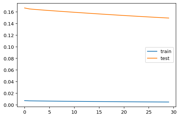

# Get the predicted values
predictions = model.predict(x_test)
predictions = scaler.inverse_transform(predictions)

1/3 [=========>....................] - ETA: 0s

3/3 [==============================] - ETA: 0s

3/3 [==============================] - 0s 31ms/step

y_test = y_test.reshape(-1,1)
y_test = scaler.inverse_transform(y_test)

# Calculate the mean absolute error (MAE)
mae = mean_absolute_error(y_test, predictions)
print('MAE: ' + str(round(mae, 1)))

# Calculate the root mean squarred error (RMSE)
rmse = np.sqrt(mean_squared_error(y_test,predictions))
print('RMSE: ' + str(round(rmse, 1)))

# Calculate the root mean squarred error (RMSE)
rmse = mean_squared_error(y_test, 
                          predictions,
                          squared = False)
print('RMSE: ' + str(round(rmse, 1)))

MAE: 1074.0
RMSE: 1479.1
RMSE: 1479.1

# Add the difference between the valid and predicted prices
train = data_asturias[:(len(x_train)+92)]
valid = data_asturias[(len(x_train)+91):]

valid.insert(1, "Predictions", predictions, True)
valid.insert(1, "Difference", valid["Predictions"] - valid["num_casos"], True)

# Zoom-in to a closer timeframe
# Date from which on the date is displayed
display_start_date = "2021-10-31" 
valid = valid[valid.index > display_start_date]
train = train[train.index > display_start_date]

# Visualize the data
matplotlib.style.use('ggplot')
fig, ax1 = plt.subplots(figsize=(22, 10), sharex=True)

# Data - Train
xt = train.index; 
yt = train[["num_casos"]]
# Data - Test / validation 
xv = valid.index; 
yv = valid[["num_casos", "Predictions"]]

# Plot
plt.title("Asturias: Predictions vs Real infections", fontsize=20)
plt.ylabel("Nº Cases", fontsize=18)

plt.plot(yt, color="blue", linewidth=1.5)
plt.plot(yv["Predictions"], color="red", linewidth=1.5)
plt.plot(yv["num_casos"], color="green", linewidth=1.5)
plt.legend(["Train", "LSTM Predictions", "Test"], 
           loc="upper left", fontsize=18)

# Bar plot with the differences
x = valid.index
y = valid["Difference"]
plt.bar(x, y, width=0.2, color="grey")
plt.grid()
plt.show()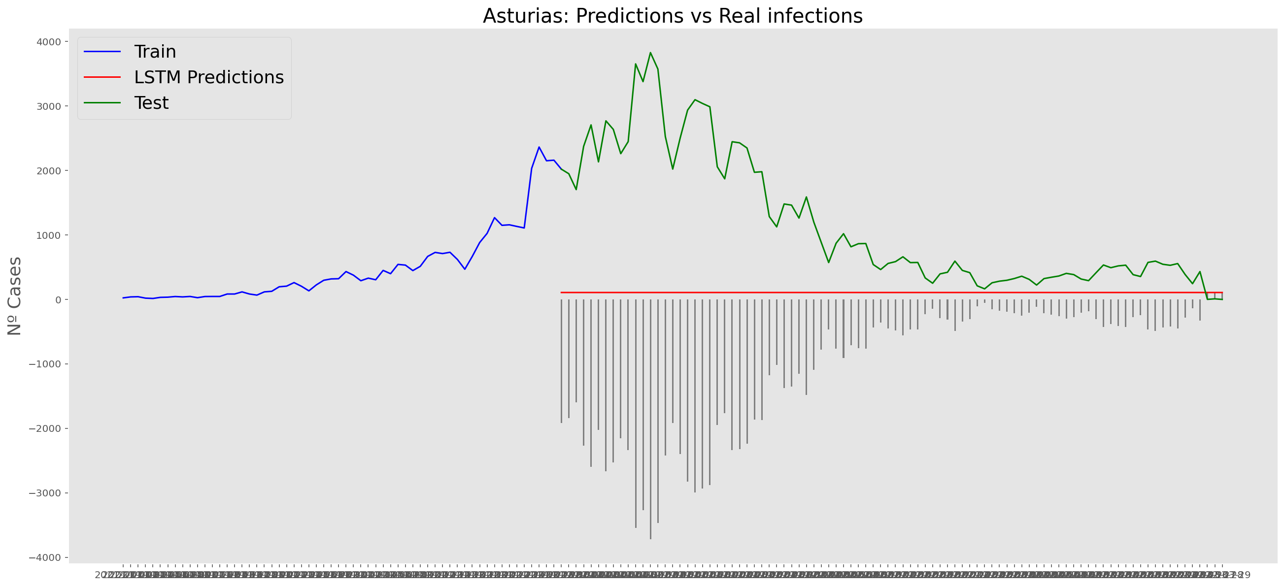

Barcelona

data_Barcelona = data_covid.loc[data_covid['provincia'] == 'Barcelona']
data_Barcelona = data_Barcelona.set_index('fecha')
data_Barcelona = data_Barcelona.filter(['num_casos'])
data_Barcelona = data_Barcelona['2020-06-14':]
data_Barcelona

	num_casos
fecha
2020-06-14	33
2020-06-15	62
2020-06-16	66
2020-06-17	70
2020-06-18	68
...	...
2022-03-25	598
2022-03-26	345
2022-03-27	252
2022-03-28	688
2022-03-29	0

654 rows × 1 columns

data_Barcelona.describe()

	num_casos
count	654.000000
mean	2605.048930
std	4823.001644
min	0.000000
25%	597.250000
50%	1030.500000
75%	2243.750000
max	34701.000000

np_data_Barcelona = data_Barcelona.values

scaler = MinMaxScaler(feature_range=(0, 1))
scaled_data_Barcelona = scaler.fit_transform(np_data_Barcelona)
print(f'Longitud del conjunto de datos disponible: {len(scaled_data_Barcelona)}')

Longitud del conjunto de datos disponible: 654

# Since we are going to predict future values based on the 90 past elements, 
# we need to create a list with those historic information for each element
historic_values = 90
scaled_data_Barcelona_x = []
scaled_data_Barcelona_y = []

for num_casos_i in range(historic_values, len(scaled_data_Barcelona)):
    scaled_data_Barcelona_x.append(scaled_data_Barcelona[(num_casos_i-historic_values):num_casos_i, 0])
    scaled_data_Barcelona_y.append(scaled_data_Barcelona[num_casos_i, 0])

# Convert the x_train and y_train to numpy arrays
scaled_data_Barcelona_x = np.array(scaled_data_Barcelona_x)
scaled_data_Barcelona_y = np.array(scaled_data_Barcelona_y)

# Train data looks like
scaled_data_Barcelona_x[235]

array([0.05037319, 0.04726089, 0.02899052, 0.02507132, 0.04639636,
       0.04190081, 0.03749171, 0.03527276, 0.03786634, 0.02619521,
       0.02351517, 0.04077692, 0.03760699, 0.03587793, 0.0364831 ,
       0.03120948, 0.02449497, 0.02083513, 0.03792398, 0.03613729,
       0.03195873, 0.02754964, 0.02818363, 0.02025878, 0.01752111,
       0.03484049, 0.03037376, 0.02870234, 0.0233999 , 0.02610876,
       0.01876027, 0.01645486, 0.0282989 , 0.02625285, 0.02680038,
       0.02564768, 0.02596467, 0.01953834, 0.01746347, 0.03184346,
       0.02973978, 0.02573413, 0.02838535, 0.02919224, 0.02190139,
       0.01890435, 0.03720354, 0.03642546, 0.0325639 , 0.0304314 ,
       0.03556093, 0.02524423, 0.02149794, 0.03803925, 0.03426414,
       0.03048903, 0.03365897, 0.02218956, 0.02530186, 0.02533068,
       0.02832771, 0.03835624, 0.03740526, 0.03512867, 0.03680009,
       0.02855825, 0.02118095, 0.03878851, 0.03507104, 0.03985476,
       0.03155529, 0.03394715, 0.02423561, 0.02169966, 0.03953777,
       0.04596409, 0.0350134 , 0.0395954 , 0.03267917, 0.02772254,
       0.02380335, 0.04668453, 0.04213135, 0.03806807, 0.03671364,
       0.03509985, 0.02106568, 0.01694476, 0.03803925, 0.02815481])

# Test data looks like
scaled_data_Barcelona_y[235]

0.030661940578081325

# Since the first 90th values does not have historic, the dataset has been reduced in 90 values
print(f'Longitud datos de entrenamiento con historico: {len(scaled_data_Barcelona_y)}')

Longitud datos de entrenamiento con historico: 564

# we split data in train and test
# as in previous analysis, we are going to predict a maximum of 90 days
x_train = scaled_data_Barcelona_x[0:len(scaled_data_Barcelona_x)-91]
y_train = scaled_data_Barcelona_y[0:len(scaled_data_Barcelona_y)-91]
print(f'Cantidad datos de entrenamiento: x={len(x_train)} - y={len(y_train)}')

x_test = scaled_data_Barcelona_x[len(scaled_data_Barcelona_x)-90:len(scaled_data_Barcelona_x)]
y_test = scaled_data_Barcelona_y[len(scaled_data_Barcelona_y)-90:len(scaled_data_Barcelona_y)]
print(f'Cantidad datos de test: x={len(x_test)} - y={len(y_test)}')

Cantidad datos de entrenamiento: x=473 - y=473
Cantidad datos de test: x=90 - y=90

# Reshape the data to feed de recurrent network
x_train = np.reshape(x_train, (x_train.shape[0], x_train.shape[1], 1))
print("Train data shape:")
print(x_train.shape)
print(y_train.shape)
x_test = np.reshape(x_test, (x_test.shape[0], x_test.shape[1], 1))
print("Test data shape:")
print(x_test.shape)
print(y_test.shape)

Train data shape:
(473, 90, 1)
(473,)
Test data shape:
(90, 90, 1)
(90,)

# Configure / setup the neural network model - LSTM
# Build the model
print('Build model...')
model = Sequential()
# Model with Neurons 
# Inputshape = neurons -> Timestamps
neurons= x_train.shape[1]
model.add(LSTM(90, 
               activation = 'relu',
               return_sequences = True, 
               input_shape = (x_train.shape[1], 1))) 
model.add(LSTM(50, 
               activation = 'relu',
               return_sequences = True)) 
model.add(LSTM(25, 
               activation = 'relu',
               return_sequences = False)) 
model.add(Dense(5, activation = 'relu'))
model.add(Dense(1))

Build model...

model.compile(optimizer='adam', loss='mean_squared_error')
model.summary()

Model: "sequential_1"

_________________________________________________________________

 Layer (type)                Output Shape              Param #

=================================================================

 lstm_3 (LSTM)               (None, 90, 90)            33120

 lstm_4 (LSTM)               (None, 90, 50)            28200

 lstm_5 (LSTM)               (None, 25)                7600

 dense_2 (Dense)             (None, 5)                 130

 dense_3 (Dense)             (None, 1)                 6

=================================================================

Total params: 69,056

Trainable params: 69,056

Non-trainable params: 0

_________________________________________________________________

# Training the model
# fit network
history = model.fit(x_train, 
                    y_train, 
                    batch_size = 1000, 
                    epochs = 30, 
                    validation_data = (x_test, y_test), 
                    verbose = 0)

plt.plot(history.history['loss'], label='train')
plt.plot(history.history['val_loss'], label='test')
plt.legend()
plt.show()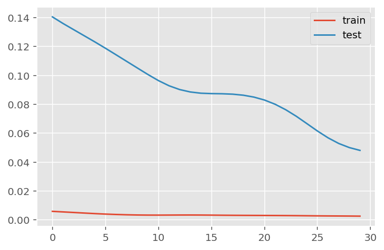

# Get the predicted values
predictions = model.predict(x_test)
predictions = scaler.inverse_transform(predictions)

1/3 [=========>....................] - ETA: 0s

3/3 [==============================] - ETA: 0s

3/3 [==============================] - 0s 31ms/step

y_test = y_test.reshape(-1,1)
y_test = scaler.inverse_transform(y_test)

# Calculate the mean absolute error (MAE)
mae = mean_absolute_error(y_test, predictions)
print('MAE: ' + str(round(mae, 1)))

# Calculate the root mean squarred error (RMSE)
rmse = np.sqrt(mean_squared_error(y_test,predictions))
print('RMSE: ' + str(round(rmse, 1)))

# Calculate the root mean squarred error (RMSE)
rmse = mean_squared_error(y_test, 
                          predictions,
                          squared = False)
print('RMSE: ' + str(round(rmse, 1)))

MAE: 5228.7
RMSE: 7609.8
RMSE: 7609.8

# Add the difference between the valid and predicted prices
train = data_Barcelona[:(len(x_train)+92)]
valid = data_Barcelona[(len(x_train)+91):]

valid.insert(1, "Predictions", predictions, True)
valid.insert(1, "Difference", valid["Predictions"] - valid["num_casos"], True)

# Zoom-in to a closer timeframe
# Date from which on the date is displayed
display_start_date = "2021-10-31" 
valid = valid[valid.index > display_start_date]
train = train[train.index > display_start_date]

# Visualize the data
matplotlib.style.use('ggplot')
fig, ax1 = plt.subplots(figsize=(22, 10), sharex=True)

# Data - Train
xt = train.index; 
yt = train[["num_casos"]]
# Data - Test / validation 
xv = valid.index; 
yv = valid[["num_casos", "Predictions"]]

# Plot
plt.title("Barcelona: Predictions vs Real infections", fontsize=20)
plt.ylabel("Nº Cases", fontsize=18)

plt.plot(yt, color="blue", linewidth=1.5)
plt.plot(yv["Predictions"], color="red", linewidth=1.5)
plt.plot(yv["num_casos"], color="green", linewidth=1.5)
plt.legend(["Train", "LSTM Predictions", "Test"], 
           loc="upper left", fontsize=18)

# Bar plot with the differences
x = valid.index
y = valid["Difference"]
plt.bar(x, y, width=0.2, color="grey")
plt.grid()
plt.show()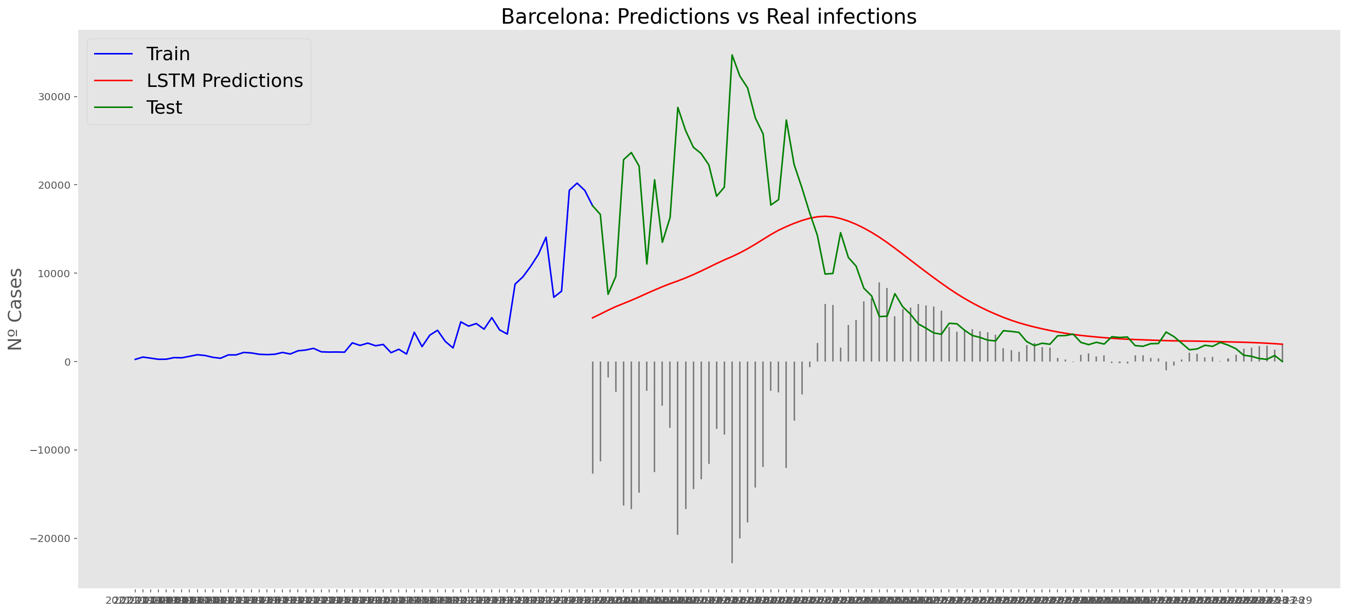

Madrid

data_Madrid = data_covid.loc[data_covid['provincia'] == 'Madrid']
data_Madrid = data_Madrid.set_index('fecha')
data_Madrid = data_Madrid.filter(['num_casos'])
data_Madrid = data_Madrid['2020-06-14':]
data_Madrid

	num_casos
fecha
2020-06-14	81
2020-06-15	153
2020-06-16	91
2020-06-17	93
2020-06-18	85
...	...
2022-03-25	356
2022-03-26	303
2022-03-27	77
2022-03-28	839
2022-03-29	6

654 rows × 1 columns

data_Madrid.describe()

	num_casos
count	654.000000
mean	2392.562691
std	3390.272836
min	6.000000
25%	662.750000
50%	1413.000000
75%	2475.750000
max	23811.000000

np_data_Madrid = data_Madrid.values

scaler = MinMaxScaler(feature_range=(0, 1))
scaled_data_Madrid = scaler.fit_transform(np_data_Madrid)
print(f'Longitud del conjunto de datos disponible: {len(scaled_data_Madrid)}')

Longitud del conjunto de datos disponible: 654

# Since we are going to predict future values based on the X past elements, 
# we need to create a list with those historic information for each element
historic_values = 90
scaled_data_Madrid_x = []
scaled_data_Madrid_y = []

for num_casos_i in range(historic_values, len(scaled_data_Madrid)):
    scaled_data_Madrid_x.append(scaled_data_Madrid[(num_casos_i-historic_values):num_casos_i, 0])
    scaled_data_Madrid_y.append(scaled_data_Madrid[num_casos_i, 0])

# Convert the x_train and y_train to numpy arrays
scaled_data_Madrid_x = np.array(scaled_data_Madrid_x)
scaled_data_Madrid_y = np.array(scaled_data_Madrid_y)

# Train data looks like
scaled_data_Madrid_x[235]

array([0.11510187, 0.14820416, 0.08880487, 0.06481832, 0.11169922,
       0.11354757, 0.089477  , 0.0694812 , 0.09300567, 0.06133165,
       0.04709095, 0.08447805, 0.07746272, 0.06595253, 0.05708885,
       0.06515438, 0.04835119, 0.04377232, 0.06372611, 0.05931527,
       0.05141777, 0.04541063, 0.05330813, 0.04150389, 0.04032766,
       0.05486242, 0.05225793, 0.04822516, 0.04259609, 0.05246797,
       0.03919345, 0.03860534, 0.05561857, 0.05452636, 0.04814115,
       0.04448645, 0.05288805, 0.04125184, 0.03994959, 0.05448435,
       0.05183785, 0.0531401 , 0.05713085, 0.0431842 , 0.05061962,
       0.0478891 , 0.07292586, 0.07830288, 0.0626339 , 0.05902121,
       0.07485822, 0.05326612, 0.05335014, 0.07111951, 0.07095148,
       0.07784079, 0.05469439, 0.06166772, 0.07149758, 0.07456417,
       0.09880277, 0.09850872, 0.0857803 , 0.08178954, 0.08951901,
       0.07225373, 0.05977736, 0.09750053, 0.09762655, 0.08930897,
       0.08544423, 0.09489603, 0.07187566, 0.06406217, 0.09329973,
       0.09855072, 0.08435203, 0.07653854, 0.08905692, 0.0647343 ,
       0.05486242, 0.08237765, 0.0873766 , 0.07326192, 0.06259189,
       0.07485822, 0.04654484, 0.04494854, 0.04721697, 0.06700273])

# Test data looks like
scaled_data_Madrid_y[235]

0.0648183154799412

# Since the first 90th values does not have historic, the dataset has been reduced in 90 values
print(f'Longitud datos de entrenamiento con historico: {len(scaled_data_Madrid_y)}')

Longitud datos de entrenamiento con historico: 564

# we split data in train and test
# as in previous analysis, we are going to predict a maximum of 91 days
x_train = scaled_data_Madrid_x[0:len(scaled_data_Madrid_x)-91]
y_train = scaled_data_Madrid_y[0:len(scaled_data_Madrid_y)-91]
print(f'Cantidad datos de entrenamiento: x={len(x_train)} - y={len(y_train)}')

x_test = scaled_data_Madrid_x[len(scaled_data_Madrid_x)-90:len(scaled_data_Madrid_x)]
y_test = scaled_data_Madrid_y[len(scaled_data_Madrid_y)-90:len(scaled_data_Madrid_y)]
print(f'Cantidad datos de test: x={len(x_test)} - y={len(y_test)}')

Cantidad datos de entrenamiento: x=473 - y=473
Cantidad datos de test: x=90 - y=90

# Reshape the data to feed de recurrent network
x_train = np.reshape(x_train, (x_train.shape[0], x_train.shape[1], 1))
print("Train data shape:")
print(x_train.shape)
print(y_train.shape)
x_test = np.reshape(x_test, (x_test.shape[0], x_test.shape[1], 1))
print("Test data shape:")
print(x_test.shape)
print(y_test.shape)

Train data shape:
(473, 90, 1)
(473,)
Test data shape:
(90, 90, 1)
(90,)

# Configure / setup the neural network model - LSTM
# Build the model
print('Build model...')
model = Sequential()
# Model with Neurons 
# Inputshape = neurons -> Timestamps
neurons= x_train.shape[1]
model.add(LSTM(90, 
               activation = 'relu',
               return_sequences = True, 
               input_shape = (x_train.shape[1], 1))) 
model.add(LSTM(50, 
               activation = 'relu',
               return_sequences = True)) 
model.add(LSTM(25, 
               activation = 'relu',
               return_sequences = False)) 
model.add(Dense(5, activation = 'relu'))
model.add(Dense(1))

Build model...

model.compile(optimizer='adam', loss='mean_squared_error')
model.summary()

Model: "sequential_2"

_________________________________________________________________

 Layer (type)                Output Shape              Param #

=================================================================

 lstm_6 (LSTM)               (None, 90, 90)            33120

 lstm_7 (LSTM)               (None, 90, 50)            28200

 lstm_8 (LSTM)               (None, 25)                7600

 dense_4 (Dense)             (None, 5)                 130

 dense_5 (Dense)             (None, 1)                 6

=================================================================

Total params: 69,056

Trainable params: 69,056

Non-trainable params: 0

_________________________________________________________________

# Training the model
# fit network
history = model.fit(x_train, 
                    y_train, 
                    batch_size = 1000, 
                    epochs = 30, 
                    validation_data = (x_test, y_test), 
                    verbose = 0)

plt.plot(history.history['loss'], label='train')
plt.plot(history.history['val_loss'], label='test')
plt.legend()
plt.show()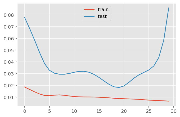

# Get the predicted values
predictions = model.predict(x_test)
predictions = scaler.inverse_transform(predictions)

1/3 [=========>....................] - ETA: 0s

3/3 [==============================] - ETA: 0s

3/3 [==============================] - 0s 30ms/step

y_test = y_test.reshape(-1,1)
y_test = scaler.inverse_transform(y_test)

# Calculate the mean absolute error (MAE)
mae = mean_absolute_error(y_test, predictions)
print('MAE: ' + str(round(mae, 1)))

# Calculate the root mean squarred error (RMSE)
rmse = np.sqrt(mean_squared_error(y_test,predictions))
print('RMSE: ' + str(round(rmse, 1)))

# Calculate the root mean squarred error (RMSE)
rmse = mean_squared_error(y_test, 
                          predictions,
                          squared = False)
print('RMSE: ' + str(round(rmse, 1)))

MAE: 4748.2
RMSE: 6975.8
RMSE: 6975.8

# Add the difference between the valid and predicted prices
train = data_Madrid[:(len(x_train)+92)]
valid = data_Madrid[(len(x_train)+91):]

valid.insert(1, "Predictions", predictions, True)
valid.insert(1, "Difference", valid["Predictions"] - valid["num_casos"], True)

# Zoom-in to a closer timeframe
# Date from which on the date is displayed
display_start_date = "2021-10-31" 
valid = valid[valid.index > display_start_date]
train = train[train.index > display_start_date]

# Visualize the data
matplotlib.style.use('ggplot')
fig, ax1 = plt.subplots(figsize=(22, 10), sharex=True)

# Data - Train
xt = train.index; 
yt = train[["num_casos"]]
# Data - Test / validation 
xv = valid.index; 
yv = valid[["num_casos", "Predictions"]]

# Plot
plt.title("Madrid: Predictions vs Real infections", fontsize=20)
plt.ylabel("Nº Cases", fontsize=18)

plt.plot(yt, color="blue", linewidth=1.5)
plt.plot(yv["Predictions"], color="red", linewidth=1.5)
plt.plot(yv["num_casos"], color="green", linewidth=1.5)
plt.legend(["Train", "LSTM Predictions", "Test"], 
           loc="upper left", fontsize=18)

# Bar plot with the differences
x = valid.index
y = valid["Difference"]
plt.bar(x, y, width=0.2, color="grey")
plt.grid()
plt.show()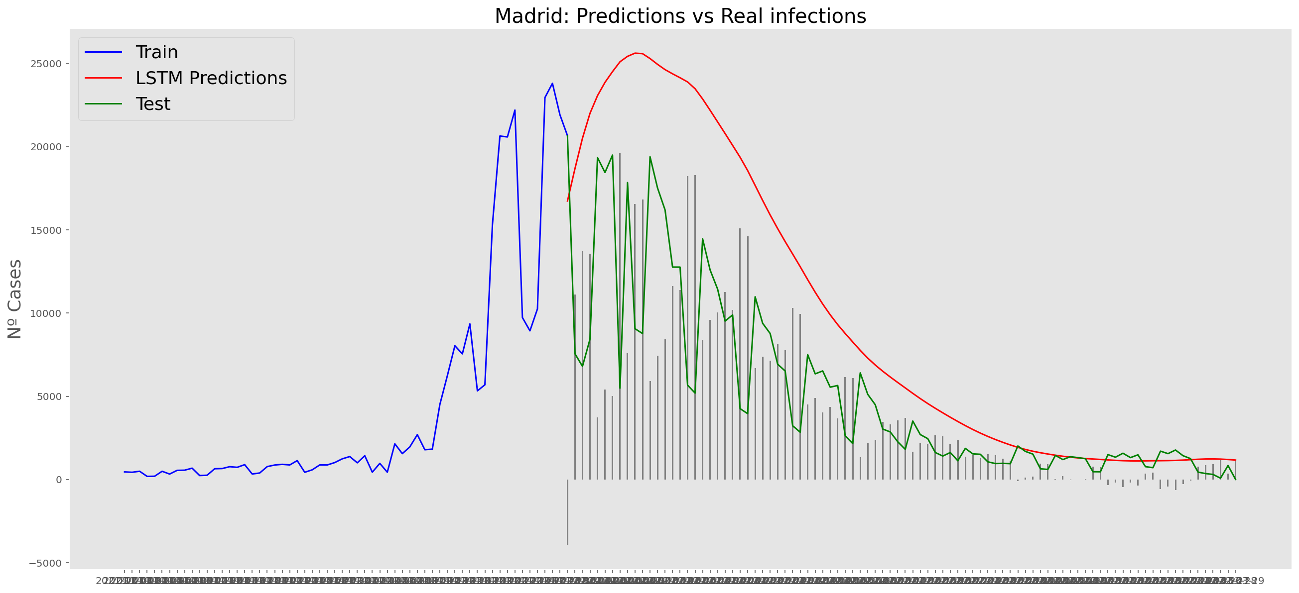

Malaga

data_Malaga = data_covid.loc[data_covid['provincia'] == 'Málaga']
data_Malaga = data_Malaga.set_index('fecha')
data_Malaga = data_Malaga.filter(['num_casos'])
data_Malaga = data_Malaga['2020-06-14':]
data_Malaga

	num_casos
fecha
2020-06-14	2
2020-06-15	1
2020-06-16	1
2020-06-17	2
2020-06-18	2
...	...
2022-03-25	565
2022-03-26	79
2022-03-27	65
2022-03-28	39
2022-03-29	0

654 rows × 1 columns

data_Malaga.describe()

	num_casos
count	654.000000
mean	410.206422
std	489.452348
min	0.000000
25%	122.250000
50%	215.500000
75%	475.250000
max	3080.000000

np_data_Malaga = data_Malaga.values

scaler = MinMaxScaler(feature_range=(0, 1))
scaled_data_Malaga = scaler.fit_transform(np_data_Malaga)
print(f'Longitud del conjunto de datos disponible: {len(scaled_data_Malaga)}')

Longitud del conjunto de datos disponible: 654

# Since we are going to predict future values based on the X past elements, 
# we need to create a list with those historic information for each element
historic_values = 90
scaled_data_Malaga_x = []
scaled_data_Malaga_y = []

for num_casos_i in range(historic_values, len(scaled_data_Malaga)):
    scaled_data_Malaga_x.append(scaled_data_Malaga[(num_casos_i-historic_values):num_casos_i, 0])
    scaled_data_Malaga_y.append(scaled_data_Malaga[num_casos_i, 0])

# Convert the x_train and y_train to numpy arrays
scaled_data_Malaga_x = np.array(scaled_data_Malaga_x)
scaled_data_Malaga_y = np.array(scaled_data_Malaga_y)

# Train data looks like
scaled_data_Malaga_x[235]

array([0.24448052, 0.21915584, 0.15649351, 0.12045455, 0.15357143,
       0.14448052, 0.1474026 , 0.14675325, 0.11655844, 0.09448052,
       0.06753247, 0.09545455, 0.11071429, 0.06883117, 0.06980519,
       0.06688312, 0.04902597, 0.03474026, 0.05974026, 0.04935065,
       0.04967532, 0.04480519, 0.04188312, 0.03993506, 0.02954545,
       0.04188312, 0.04772727, 0.05162338, 0.04902597, 0.04318182,
       0.02792208, 0.0288961 , 0.04253247, 0.04123377, 0.04025974,
       0.03538961, 0.05097403, 0.03051948, 0.02662338, 0.04123377,
       0.03149351, 0.04350649, 0.03733766, 0.03571429, 0.02954545,
       0.0211039 , 0.04188312, 0.04545455, 0.03863636, 0.04772727,
       0.04935065, 0.03571429, 0.0288961 , 0.05357143, 0.05324675,
       0.05616883, 0.04253247, 0.04058442, 0.03474026, 0.04935065,
       0.06623377, 0.07824675, 0.06623377, 0.05909091, 0.06233766,
       0.05064935, 0.03116883, 0.07077922, 0.05649351, 0.07792208,
       0.06168831, 0.0711039 , 0.04155844, 0.04577922, 0.06623377,
       0.06720779, 0.05909091, 0.05519481, 0.05324675, 0.04383117,
       0.03668831, 0.05941558, 0.06525974, 0.06006494, 0.05551948,
       0.05876623, 0.04512987, 0.04545455, 0.06266234, 0.07727273])

# Test data looks like
scaled_data_Malaga_y[235]

0.0737012987012987

# Since the first 90th values does not have historic, the dataset has been reduced in 90 values
print(f'Longitud datos de entrenamiento con historico: {len(scaled_data_Malaga_y)}')

Longitud datos de entrenamiento con historico: 564

# we split data in train and test
# as in previous analysis, we are going to predict a maximum of 91 days
x_train = scaled_data_Malaga_x[0:len(scaled_data_Malaga_x)-91]
y_train = scaled_data_Malaga_y[0:len(scaled_data_Malaga_y)-91]
print(f'Cantidad datos de entrenamiento: x={len(x_train)} - y={len(y_train)}')

x_test = scaled_data_Malaga_x[len(scaled_data_Malaga_x)-90:len(scaled_data_Malaga_x)]
y_test = scaled_data_Malaga_y[len(scaled_data_Malaga_y)-90:len(scaled_data_Malaga_y)]
print(f'Cantidad datos de test: x={len(x_test)} - y={len(y_test)}')

Cantidad datos de entrenamiento: x=473 - y=473
Cantidad datos de test: x=90 - y=90

# Reshape the data to feed de recurrent network
x_train = np.reshape(x_train, (x_train.shape[0], x_train.shape[1], 1))
print("Train data shape:")
print(x_train.shape)
print(y_train.shape)
x_test = np.reshape(x_test, (x_test.shape[0], x_test.shape[1], 1))
print("Test data shape:")
print(x_test.shape)
print(y_test.shape)

Train data shape:
(473, 90, 1)
(473,)
Test data shape:
(90, 90, 1)
(90,)

# Configure / setup the neural network model - LSTM
# Build the model
print('Build model...')
model = Sequential()
# Model with Neurons 
# Inputshape = neurons -> Timestamps
neurons= x_train.shape[1]
model.add(LSTM(90, 
               activation = 'relu',
               return_sequences = True, 
               input_shape = (x_train.shape[1], 1))) 
model.add(LSTM(50, 
               activation = 'relu',
               return_sequences = True)) 
model.add(LSTM(25, 
               activation = 'relu',
               return_sequences = False)) 
model.add(Dense(5, activation = 'relu'))
model.add(Dense(1))

Build model...

model.compile(optimizer='adam', loss='mean_squared_error')
model.summary()

Model: "sequential_3"

_________________________________________________________________

 Layer (type)                Output Shape              Param #

=================================================================

 lstm_9 (LSTM)               (None, 90, 90)            33120

 lstm_10 (LSTM)              (None, 90, 50)            28200

 lstm_11 (LSTM)              (None, 25)                7600

 dense_6 (Dense)             (None, 5)                 130

 dense_7 (Dense)             (None, 1)                 6

=================================================================

Total params: 69,056

Trainable params: 69,056

Non-trainable params: 0

_________________________________________________________________

# Training the model
# fit network
history = model.fit(x_train, 
                    y_train, 
                    batch_size = 1000, 
                    epochs = 30, 
                    validation_data = (x_test, y_test), 
                    verbose = 0)

plt.plot(history.history['loss'], label='train')
plt.plot(history.history['val_loss'], label='test')
plt.legend()
plt.show()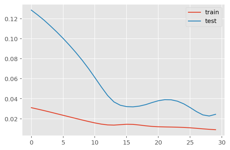

# Get the predicted values
predictions = model.predict(x_test)
predictions = scaler.inverse_transform(predictions)

1/3 [=========>....................] - ETA: 0s

3/3 [==============================] - ETA: 0s

3/3 [==============================] - 0s 31ms/step

y_test = y_test.reshape(-1,1)
y_test = scaler.inverse_transform(y_test)

# Calculate the mean absolute error (MAE)
mae = mean_absolute_error(y_test, predictions)
print('MAE: ' + str(round(mae, 1)))

# Calculate the root mean squarred error (RMSE)
rmse = np.sqrt(mean_squared_error(y_test,predictions))
print('RMSE: ' + str(round(rmse, 1)))

# Calculate the root mean squarred error (RMSE)
rmse = mean_squared_error(y_test, 
                          predictions,
                          squared = False)
print('RMSE: ' + str(round(rmse, 1)))

MAE: 353.5
RMSE: 481.1
RMSE: 481.1

# Add the difference between the valid and predicted prices
train = data_Malaga[:(len(x_train)+92)]
valid = data_Malaga[(len(x_train)+91):]

valid.insert(1, "Predictions", predictions, True)
valid.insert(1, "Difference", valid["Predictions"] - valid["num_casos"], True)

# Zoom-in to a closer timeframe
# Date from which on the date is displayed
display_start_date = "2021-10-31" 
valid = valid[valid.index > display_start_date]
train = train[train.index > display_start_date]

# Visualize the data
matplotlib.style.use('ggplot')
fig, ax1 = plt.subplots(figsize=(22, 10), sharex=True)

# Data - Train
xt = train.index; 
yt = train[["num_casos"]]
# Data - Test / validation 
xv = valid.index; 
yv = valid[["num_casos", "Predictions"]]

# Plot
plt.title("Malaga: Predictions vs Real infections", fontsize=20)
plt.ylabel("Nº Cases", fontsize=18)

plt.plot(yt, color="blue", linewidth=1.5)
plt.plot(yv["Predictions"], color="red", linewidth=1.5)
plt.plot(yv["num_casos"], color="green", linewidth=1.5)
plt.legend(["Train", "LSTM Predictions", "Test"], 
           loc="upper left", fontsize=18)

# Bar plot with the differences
x = valid.index
y = valid["Difference"]
plt.bar(x, y, width=0.2, color="grey")
plt.grid()
plt.show()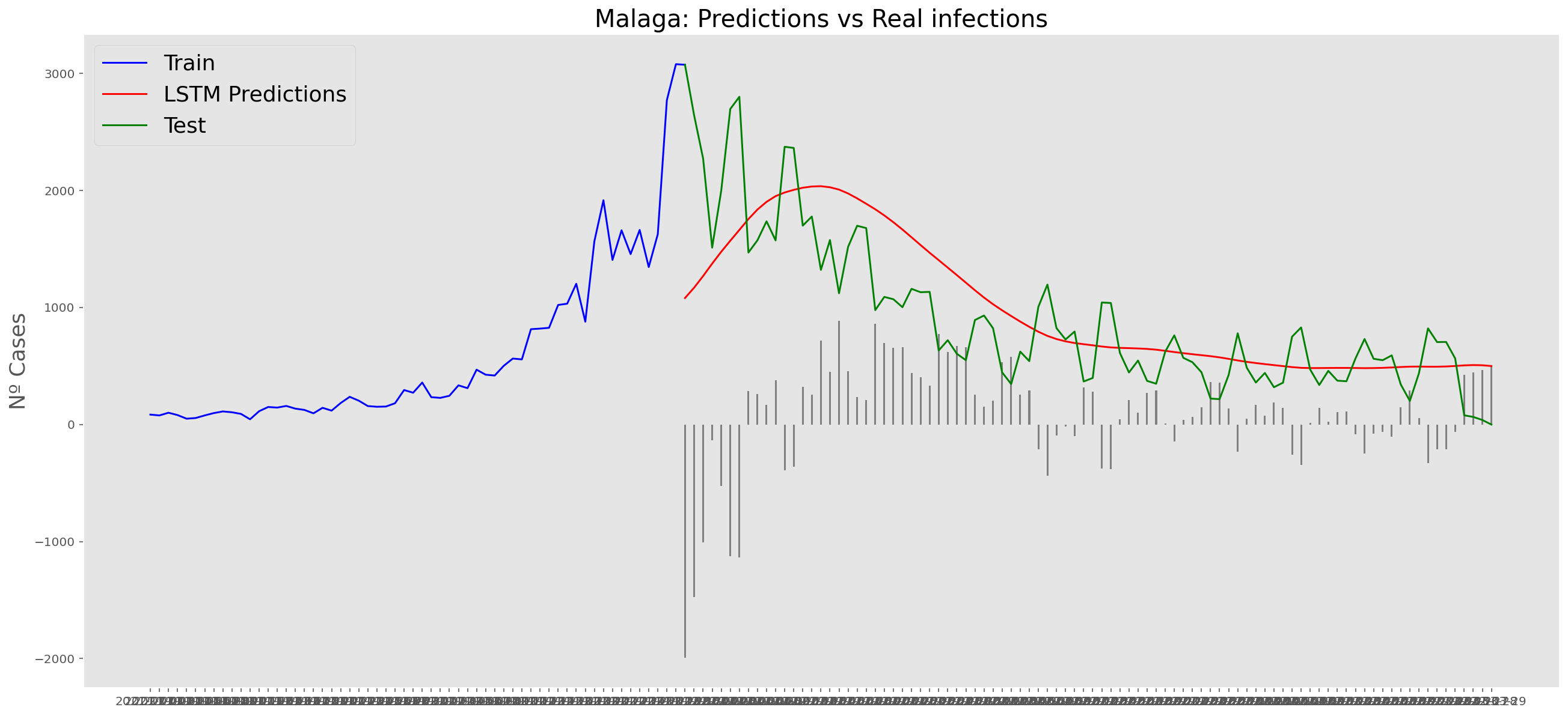

Sevilla

data_Sevilla = data_covid.loc[data_covid['provincia'] == 'Sevilla']
data_Sevilla = data_Sevilla.set_index('fecha')
data_Sevilla = data_Sevilla.filter(['num_casos'])
data_Sevilla = data_Sevilla['2020-06-14':]
data_Sevilla

	num_casos
fecha
2020-06-14	0
2020-06-15	2
2020-06-16	1
2020-06-17	0
2020-06-18	0
...	...
2022-03-25	365
2022-03-26	67
2022-03-27	24
2022-03-28	12
2022-03-29	0

654 rows × 1 columns

data_Sevilla.describe()

	num_casos
count	654.000000
mean	432.978593
std	500.618517
min	0.000000
25%	127.250000
50%	282.000000
75%	528.250000
max	3692.000000

np_data_Sevilla = data_Sevilla.values

scaler = MinMaxScaler(feature_range=(0, 1))
scaled_data_Sevilla = scaler.fit_transform(np_data_Sevilla)
print(f'Longitud del conjunto de datos disponible: {len(scaled_data_Sevilla)}')

Longitud del conjunto de datos disponible: 654

# Since we are going to predict future values based on the X past elements, 
# we need to create a list with those historic information for each element
historic_values = 90
scaled_data_Sevilla_x = []
scaled_data_Sevilla_y = []

for num_casos_i in range(historic_values, len(scaled_data_Sevilla)):
    scaled_data_Sevilla_x.append(scaled_data_Sevilla[(num_casos_i-historic_values):num_casos_i, 0])
    scaled_data_Sevilla_y.append(scaled_data_Sevilla[num_casos_i, 0])

# Convert the x_train and y_train to numpy arrays
scaled_data_Sevilla_x = np.array(scaled_data_Sevilla_x)
scaled_data_Sevilla_y = np.array(scaled_data_Sevilla_y)

# Train data looks like
scaled_data_Sevilla_x[235]

array([0.18634886, 0.19799567, 0.14626219, 0.0896533 , 0.13894908,
       0.1695558 , 0.14572048, 0.12242687, 0.13434453, 0.06500542,
       0.05390033, 0.08206934, 0.08667389, 0.09452871, 0.06798483,
       0.05904659, 0.04252438, 0.0343987 , 0.06554713, 0.06473456,
       0.05444204, 0.0503792 , 0.05796316, 0.04577465, 0.03819068,
       0.04712893, 0.0528169 , 0.0663597 , 0.06013001, 0.05119177,
       0.03764897, 0.031961  , 0.05119177, 0.05010834, 0.04739978,
       0.05119177, 0.05390033, 0.03927411, 0.03737811, 0.06013001,
       0.05633803, 0.05606717, 0.05850488, 0.06473456, 0.04658722,
       0.04198267, 0.07150596, 0.07340195, 0.05823402, 0.08071506,
       0.07773564, 0.05877573, 0.05471289, 0.07990249, 0.08829902,
       0.0872156 , 0.09019502, 0.07069339, 0.08775731, 0.08396533,
       0.14951246, 0.12432286, 0.12269772, 0.12378115, 0.13028169,
       0.11348862, 0.07936078, 0.13299025, 0.12269772, 0.11213434,
       0.12107259, 0.12432286, 0.09723727, 0.07042254, 0.09886241,
       0.11782232, 0.10157096, 0.10346696, 0.12621885, 0.08342362,
       0.07340195, 0.0847779 , 0.08559047, 0.11159263, 0.10292524,
       0.08911159, 0.07502709, 0.04821235, 0.08315276, 0.09913326])

# Test data looks like
scaled_data_Sevilla_y[235]

0.10861321776814734

# Since the first 90th values does not have historic, the dataset has been reduced in 90 values
print(f'Longitud datos de entrenamiento con historico: {len(scaled_data_Sevilla_y)}')

Longitud datos de entrenamiento con historico: 564

# we split data in train and test
# as in previous analysis, we are going to predict a maximum of 91 days
x_train = scaled_data_Sevilla_x[0:len(scaled_data_Sevilla_x)-91]
y_train = scaled_data_Sevilla_y[0:len(scaled_data_Sevilla_y)-91]
print(f'Cantidad datos de entrenamiento: x={len(x_train)} - y={len(y_train)}')

x_test = scaled_data_Sevilla_x[len(scaled_data_Sevilla_x)-90:len(scaled_data_Sevilla_x)]
y_test = scaled_data_Sevilla_y[len(scaled_data_Sevilla_y)-90:len(scaled_data_Sevilla_y)]
print(f'Cantidad datos de test: x={len(x_test)} - y={len(y_test)}')

Cantidad datos de entrenamiento: x=473 - y=473
Cantidad datos de test: x=90 - y=90

# Reshape the data to feed de recurrent network
x_train = np.reshape(x_train, (x_train.shape[0], x_train.shape[1], 1))
print("Train data shape:")
print(x_train.shape)
print(y_train.shape)
x_test = np.reshape(x_test, (x_test.shape[0], x_test.shape[1], 1))
print("Test data shape:")
print(x_test.shape)
print(y_test.shape)

Train data shape:
(473, 90, 1)
(473,)
Test data shape:
(90, 90, 1)
(90,)

# Configure / setup the neural network model - LSTM
# Build the model
print('Build model...')
model = Sequential()
# Model with Neurons 
# Inputshape = neurons -> Timestamps
neurons= x_train.shape[1]
model.add(LSTM(90, 
               activation = 'relu',
               return_sequences = True, 
               input_shape = (x_train.shape[1], 1))) 
model.add(LSTM(50, 
               activation = 'relu',
               return_sequences = True)) 
model.add(LSTM(25, 
               activation = 'relu',
               return_sequences = False)) 
model.add(Dense(5, activation = 'relu'))
model.add(Dense(1))

Build model...

model.compile(optimizer='adam', loss='mean_squared_error')
model.summary()

Model: "sequential_4"

_________________________________________________________________

 Layer (type)                Output Shape              Param #

=================================================================

 lstm_12 (LSTM)              (None, 90, 90)            33120

 lstm_13 (LSTM)              (None, 90, 50)            28200

 lstm_14 (LSTM)              (None, 25)                7600

 dense_8 (Dense)             (None, 5)                 130

 dense_9 (Dense)             (None, 1)                 6

=================================================================

Total params: 69,056

Trainable params: 69,056

Non-trainable params: 0

_________________________________________________________________

# Training the model
# fit network
history = model.fit(x_train, 
                    y_train, 
                    batch_size = 1000, 
                    epochs = 30, 
                    validation_data = (x_test, y_test), 
                    verbose = 0)

plt.plot(history.history['loss'], label='train')
plt.plot(history.history['val_loss'], label='test')
plt.legend()
plt.show()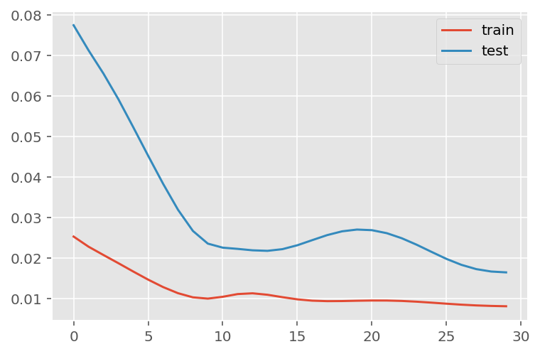

# Get the predicted values
predictions = model.predict(x_test)
predictions = scaler.inverse_transform(predictions)

WARNING:tensorflow:5 out of the last 13 calls to <function Model.make_predict_function.<locals>.predict_function at 0x7fdc69aa8c10> triggered tf.function retracing. Tracing is expensive and the excessive number of tracings could be due to (1) creating @tf.function repeatedly in a loop, (2) passing tensors with different shapes, (3) passing Python objects instead of tensors. For (1), please define your @tf.function outside of the loop. For (2), @tf.function has reduce_retracing=True option that can avoid unnecessary retracing. For (3), please refer to https://www.tensorflow.org/guide/function#controlling_retracing and https://www.tensorflow.org/api_docs/python/tf/function for  more details.

1/3 [=========>....................] - ETA: 0s

3/3 [==============================] - ETA: 0s

3/3 [==============================] - 0s 32ms/step

y_test = y_test.reshape(-1,1)
y_test = scaler.inverse_transform(y_test)

# Calculate the mean absolute error (MAE)
mae = mean_absolute_error(y_test, predictions)
print('MAE: ' + str(round(mae, 1)))

# Calculate the root mean squarred error (RMSE)
rmse = np.sqrt(mean_squared_error(y_test,predictions))
print('RMSE: ' + str(round(rmse, 1)))

# Calculate the root mean squarred error (RMSE)
rmse = mean_squared_error(y_test, 
                          predictions,
                          squared = False)
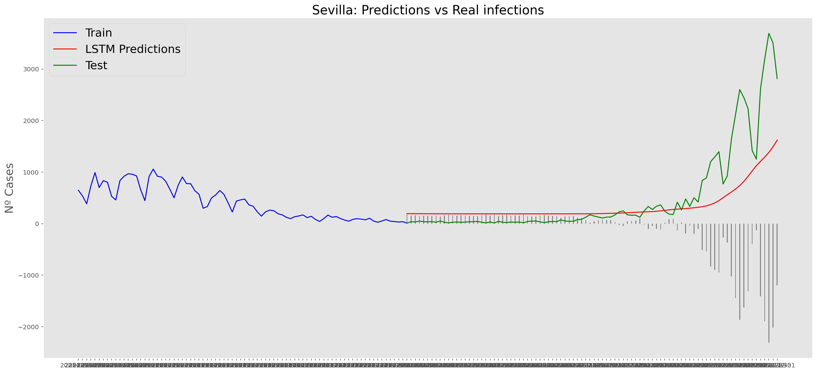
print('RMSE: ' + str(round(rmse, 1)))

MAE: 335.1
RMSE: 474.0
RMSE: 474.0

# Add the difference between the valid and predicted prices
train = data_Sevilla[:(len(x_train)+92)]
valid = data_Sevilla[(len(x_train)+91):]

valid.insert(1, "Predictions", predictions, True)
valid.insert(1, "Difference", valid["Predictions"] - valid["num_casos"], True)

# Zoom-in to a closer timeframe
# Date from which on the date is displayed
display_start_date = "2021-10-31" 
valid = valid[valid.index > display_start_date]
train = train[train.index > display_start_date]

# Visualize the data
matplotlib.style.use('ggplot')
fig, ax1 = plt.subplots(figsize=(22, 10), sharex=True)

# Data - Train
xt = train.index; 
yt = train[["num_casos"]]
# Data - Test / validation 
xv = valid.index; 
yv = valid[["num_casos", "Predictions"]]

# Plot
plt.title("Sevilla: Predictions vs Real infections", fontsize=20)
plt.ylabel("Nº Cases", fontsize=18)

plt.plot(yt, color="blue", linewidth=1.5)
plt.plot(yv["Predictions"], color="red", linewidth=1.5)
plt.plot(yv["num_casos"], color="green", linewidth=1.5)
plt.legend(["Train", "LSTM Predictions", "Test"], 
           loc="upper left", fontsize=18)

# Bar plot with the differences
x = valid.index
y = valid["Difference"]
plt.bar(x, y, width=0.2, color="grey")
plt.grid()
plt.show()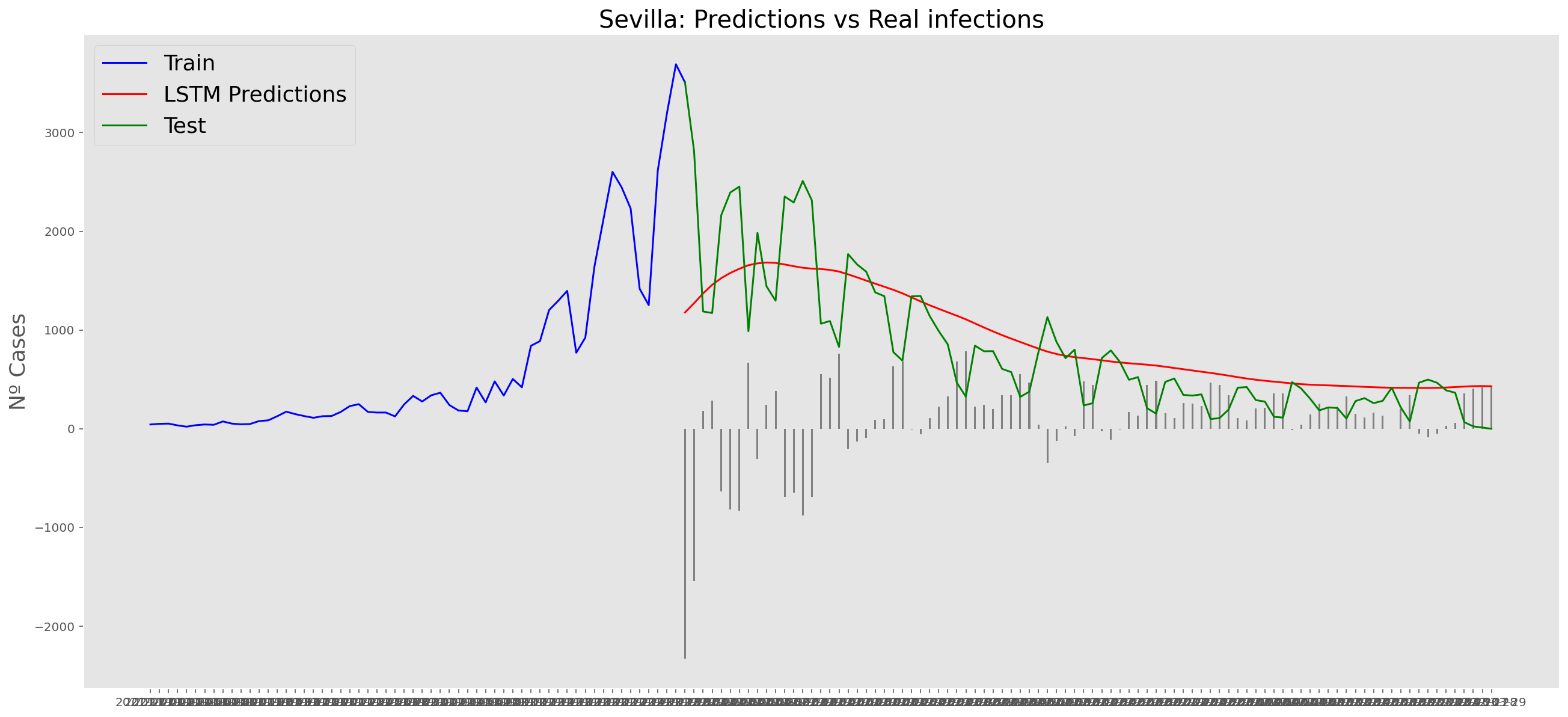

Just before the sixth wave

Asturias

data_asturias = data_covid.loc[data_covid['provincia'] == 'Asturias']
data_asturias = data_asturias.set_index('fecha')
data_asturias = data_asturias.filter(['num_casos'])
data_asturias = data_asturias['2020-06-14':'2021-12-31']
data_asturias

	num_casos
fecha
2020-06-14	0
2020-06-15	0
2020-06-16	1
2020-06-17	0
2020-06-18	0
...	...
2021-12-27	2363
2021-12-28	2150
2021-12-29	2159
2021-12-30	2020
2021-12-31	1949

566 rows × 1 columns

data_asturias.describe()

	num_casos
count	566.000000
mean	180.913428
std	276.250633
min	0.000000
25%	36.000000
50%	94.500000
75%	225.750000
max	2363.000000

np_data_asturias = data_asturias.values

scaler = MinMaxScaler(feature_range=(0, 1))
scaled_data_asturias = scaler.fit_transform(np_data_asturias)
print(f'Longitud del conjunto de datos disponible: {len(scaled_data_asturias)}')

Longitud del conjunto de datos disponible: 566

# Since we are going to predict future values based on the X past elements, 
# we need to create a list with those historic information for each element
historic_values = 90
scaled_data_asturias_x = []
scaled_data_asturias_y = []

for num_casos_i in range(historic_values, len(scaled_data_asturias)):
    scaled_data_asturias_x.append(scaled_data_asturias[(num_casos_i-historic_values):num_casos_i, 0])
    scaled_data_asturias_y.append(scaled_data_asturias[num_casos_i, 0])

# Convert the x_train and y_train to numpy arrays
scaled_data_asturias_x = np.array(scaled_data_asturias_x)
scaled_data_asturias_y = np.array(scaled_data_asturias_y)

# Since the first 90 values does not have historic, the dataset has been reduced in 90 values
print(f'Longitud datos de entrenamiento con historico: {len(scaled_data_asturias_y)}')

Longitud datos de entrenamiento con historico: 476

# we split data in train and test
# as in previous analysis, we are going to predict a maximum of 21 days
x_train = scaled_data_asturias_x[0:len(scaled_data_asturias_x)-91]
y_train = scaled_data_asturias_y[0:len(scaled_data_asturias_y)-91]
print(f'Cantidad datos de entrenamiento: x={len(x_train)} - y={len(y_train)}')

x_test = scaled_data_asturias_x[len(scaled_data_asturias_x)-90:len(scaled_data_asturias_x)]
y_test = scaled_data_asturias_y[len(scaled_data_asturias_y)-90:len(scaled_data_asturias_y)]
print(f'Cantidad datos de test: x={len(x_test)} - y={len(y_test)}')

Cantidad datos de entrenamiento: x=385 - y=385
Cantidad datos de test: x=90 - y=90

# Reshape the data to feed de recurrent network
x_train = np.reshape(x_train, (x_train.shape[0], x_train.shape[1], 1))
print("Train data shape:")
print(x_train.shape)
print(y_train.shape)
x_test = np.reshape(x_test, (x_test.shape[0], x_test.shape[1], 1))
print("Test data shape:")
print(x_test.shape)
print(y_test.shape)

Train data shape:
(385, 90, 1)
(385,)
Test data shape:
(90, 90, 1)
(90,)

# # Configure / setup the neural network model - LSTM
# Build the model
print('Build model...')
model = Sequential()
# Model with Neurons 
# Inputshape = neurons -> Timestamps
neurons= x_train.shape[1]
model.add(LSTM(90, 
               activation = 'relu',
               return_sequences = True, 
               input_shape = (x_train.shape[1], 1))) 
model.add(LSTM(50, 
               activation = 'relu',
               return_sequences = True)) 
model.add(LSTM(25, 
               activation = 'relu',
               return_sequences = False)) 
model.add(Dense(5, activation = 'relu'))
model.add(Dense(1))

Build model...

model.compile(optimizer='adam', loss='mean_squared_error')
model.summary()

Model: "sequential_5"

_________________________________________________________________

 Layer (type)                Output Shape              Param #

=================================================================

 lstm_15 (LSTM)              (None, 90, 90)            33120

 lstm_16 (LSTM)              (None, 90, 50)            28200

 lstm_17 (LSTM)              (None, 25)                7600

 dense_10 (Dense)            (None, 5)                 130

 dense_11 (Dense)            (None, 1)                 6

=================================================================

Total params: 69,056

Trainable params: 69,056

Non-trainable params: 0

_________________________________________________________________

# Training the model
# # fit network
history = model.fit(x_train, 
                    y_train, 
                    batch_size=1000, 
                    epochs=50, 
                    validation_data = (x_test, y_test), 
                    verbose = 0)

plt.plot(history.history['loss'], label='train')
plt.plot(history.history['val_loss'], label='test')
plt.legend()
plt.show()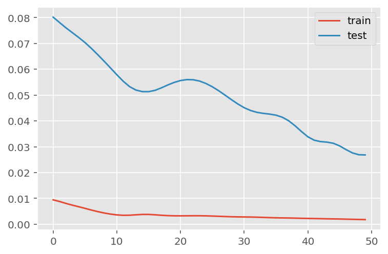

# Get the predicted values
predictions = model.predict(x_test)
predictions = scaler.inverse_transform(predictions)

WARNING:tensorflow:5 out of the last 13 calls to <function Model.make_predict_function.<locals>.predict_function at 0x7fdc3a579c10> triggered tf.function retracing. Tracing is expensive and the excessive number of tracings could be due to (1) creating @tf.function repeatedly in a loop, (2) passing tensors with different shapes, (3) passing Python objects instead of tensors. For (1), please define your @tf.function outside of the loop. For (2), @tf.function has reduce_retracing=True option that can avoid unnecessary retracing. For (3), please refer to https://www.tensorflow.org/guide/function#controlling_retracing and https://www.tensorflow.org/api_docs/python/tf/function for  more details.

1/3 [=========>....................] - ETA: 0s

3/3 [==============================] - ETA: 0s

3/3 [==============================] - 0s 31ms/step

y_test = y_test.reshape(-1,1)
y_test = scaler.inverse_transform(y_test)

# Calculate the mean absolute error (MAE)
mae = mean_absolute_error(y_test, predictions)
print('MAE: ' + str(round(mae, 1)))

# Calculate the root mean squarred error (RMSE)
rmse = np.sqrt(mean_squared_error(y_test,predictions))
print('RMSE: ' + str(round(rmse, 1)))

# Calculate the root mean squarred error (RMSE)
rmse = mean_squared_error(y_test, 
                          predictions,
                          squared = False)
print('RMSE: ' + str(round(rmse, 1)))

MAE: 208.7
RMSE: 387.0
RMSE: 387.0

# Add the difference between the valid and predicted prices
train = data_asturias[:(len(x_train)+92)]
valid = data_asturias[(len(x_train)+91):]

valid.insert(1, "Predictions", predictions, True)
valid.insert(1, "Difference", valid["Predictions"] - valid["num_casos"], True)

# Zoom-in to a closer timeframe
# Date from which on the date is displayed
display_start_date = "2021-07-15"
valid = valid[valid.index > display_start_date]
train = train[train.index > display_start_date]

# Visualize the data
matplotlib.style.use('ggplot')
fig, ax1 = plt.subplots(figsize=(22, 10), sharex=True)

# Data - Train
xt = train.index; 
yt = train[["num_casos"]]
# Data - Test / validation 
xv = valid.index; 
yv = valid[["num_casos", "Predictions"]]

# Plot
plt.title("Asturias: Predictions vs Real infections", fontsize=20)
plt.ylabel("Nº Cases", fontsize=18)

plt.plot(yt, color="blue", linewidth=1.5)
plt.plot(yv["Predictions"], color="red", linewidth=1.5)
plt.plot(yv["num_casos"], color="green", linewidth=1.5)
plt.legend(["Train", "LSTM Predictions", "Test"], 
           loc="upper left", fontsize=18)

# Bar plot with the differences
x = valid.index
y = valid["Difference"]
plt.bar(x, y, width=0.2, color="grey")
plt.grid()
plt.show()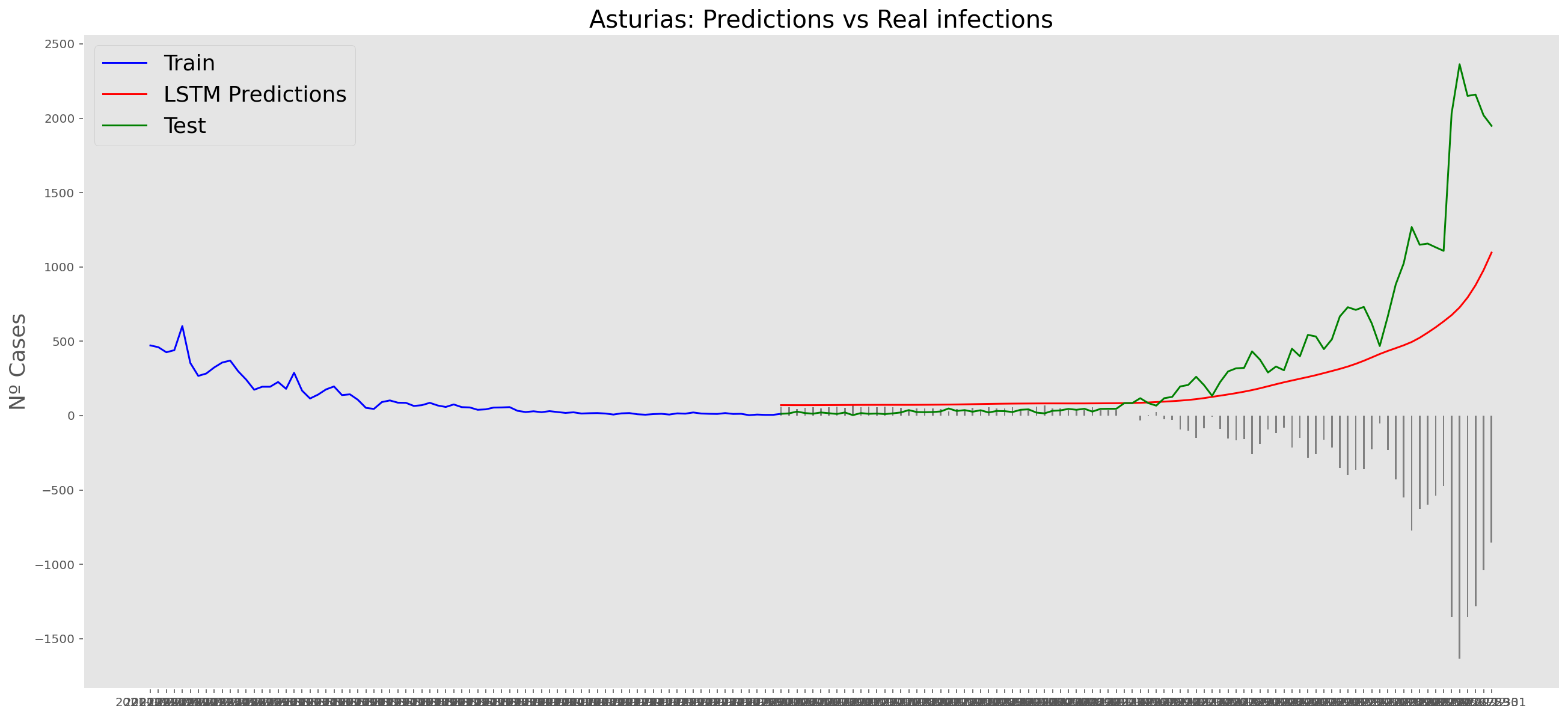

Barcelona

data_Barcelona = data_covid.loc[data_covid['provincia'] == 'Barcelona']
data_Barcelona = data_Barcelona.set_index('fecha')
data_Barcelona = data_Barcelona.filter(['num_casos'])
data_Barcelona = data_Barcelona['2020-06-14':'2021-12-31']
data_Barcelona

	num_casos
fecha
2020-06-14	33
2020-06-15	62
2020-06-16	66
2020-06-17	70
2020-06-18	68
...	...
2021-12-27	19383
2021-12-28	20192
2021-12-29	19361
2021-12-30	17639
2021-12-31	16651

566 rows × 1 columns

data_Barcelona.describe()

	num_casos
count	566.000000
mean	1575.480565
std	2281.290383
min	33.000000
25%	544.750000
50%	944.500000
75%	1609.500000
max	20192.000000

np_data_Barcelona = data_Barcelona.values

scaler = MinMaxScaler(feature_range=(0, 1))
scaled_data_Barcelona = scaler.fit_transform(np_data_Barcelona)
print(f'Longitud del conjunto de datos disponible: {len(scaled_data_Barcelona)}')

Longitud del conjunto de datos disponible: 566

# Since we are going to predict future values based on the 90 past elements, 
# we need to create a list with those historic information for each element
historic_values = 90
scaled_data_Barcelona_x = []
scaled_data_Barcelona_y = []

for num_casos_i in range(historic_values, len(scaled_data_Barcelona)):
    scaled_data_Barcelona_x.append(scaled_data_Barcelona[(num_casos_i-historic_values):num_casos_i, 0])
    scaled_data_Barcelona_y.append(scaled_data_Barcelona[num_casos_i, 0])

# Convert the x_train and y_train to numpy arrays
scaled_data_Barcelona_x = np.array(scaled_data_Barcelona_x)
scaled_data_Barcelona_y = np.array(scaled_data_Barcelona_y)

# Train data looks like
scaled_data_Barcelona_x[235]

array([0.08507366, 0.07971626, 0.04826628, 0.04151992, 0.07822809,
       0.07048961, 0.06289995, 0.05908031, 0.06354482, 0.04345454,
       0.03884121, 0.06855499, 0.06309837, 0.06012203, 0.06116375,
       0.05208592, 0.0405278 , 0.03422789, 0.06364403, 0.06056848,
       0.05337566, 0.045786  , 0.04687733, 0.03323578, 0.02852324,
       0.05833623, 0.05064735, 0.04777023, 0.03864279, 0.04330572,
       0.03065628, 0.02668783, 0.04707575, 0.04355375, 0.04449625,
       0.04251203, 0.04305769, 0.03199563, 0.02842403, 0.05317724,
       0.04955603, 0.04266085, 0.04722456, 0.04861352, 0.0360633 ,
       0.03090431, 0.06240389, 0.06106454, 0.05441738, 0.05074656,
       0.05957637, 0.04181755, 0.03536882, 0.06384245, 0.05734411,
       0.05084578, 0.0563024 , 0.03655935, 0.04191676, 0.04196637,
       0.04712535, 0.06438811, 0.06275113, 0.05883228, 0.06170941,
       0.0475222 , 0.03482316, 0.0651322 , 0.05873307, 0.06696761,
       0.05268118, 0.05679845, 0.04008135, 0.03571606, 0.06642195,
       0.077484  , 0.05863386, 0.06652116, 0.0546158 , 0.04608364,
       0.03933727, 0.07872414, 0.07088645, 0.06389206, 0.06156059,
       0.05878268, 0.03462473, 0.02753113, 0.06384245, 0.04682772])

# Test data looks like
scaled_data_Barcelona_y[235]

0.05114340989136366

# Since the first 90th values does not have historic, the dataset has been reduced in 90 values
print(f'Longitud datos de entrenamiento con historico: {len(scaled_data_Barcelona_y)}')

Longitud datos de entrenamiento con historico: 476

# we split data in train and test
# as in previous analysis, we are going to predict a maximum of 90 days
x_train = scaled_data_Barcelona_x[0:len(scaled_data_Barcelona_x)-91]
y_train = scaled_data_Barcelona_y[0:len(scaled_data_Barcelona_y)-91]
print(f'Cantidad datos de entrenamiento: x={len(x_train)} - y={len(y_train)}')

x_test = scaled_data_Barcelona_x[len(scaled_data_Barcelona_x)-90:len(scaled_data_Barcelona_x)]
y_test = scaled_data_Barcelona_y[len(scaled_data_Barcelona_y)-90:len(scaled_data_Barcelona_y)]
print(f'Cantidad datos de test: x={len(x_test)} - y={len(y_test)}')

Cantidad datos de entrenamiento: x=385 - y=385
Cantidad datos de test: x=90 - y=90

# Reshape the data to feed de recurrent network
x_train = np.reshape(x_train, (x_train.shape[0], x_train.shape[1], 1))
print("Train data shape:")
print(x_train.shape)
print(y_train.shape)
x_test = np.reshape(x_test, (x_test.shape[0], x_test.shape[1], 1))
print("Test data shape:")
print(x_test.shape)
print(y_test.shape)

Train data shape:
(385, 90, 1)
(385,)
Test data shape:
(90, 90, 1)
(90,)

# Configure / setup the neural network model - LSTM
# Build the model
print('Build model...')
model = Sequential()
# Model with Neurons 
# Inputshape = neurons -> Timestamps
neurons= x_train.shape[1]
model.add(LSTM(90, 
               activation = 'relu',
               return_sequences = True, 
               input_shape = (x_train.shape[1], 1))) 
model.add(LSTM(50, 
               activation = 'relu',
               return_sequences = True)) 
model.add(LSTM(25, 
               activation = 'relu',
               return_sequences = False)) 
model.add(Dense(5, activation = 'relu'))
model.add(Dense(1))

Build model...

model.compile(optimizer='adam', loss='mean_squared_error')
model.summary()

Model: "sequential_6"

_________________________________________________________________

 Layer (type)                Output Shape              Param #

=================================================================

 lstm_18 (LSTM)              (None, 90, 90)            33120

 lstm_19 (LSTM)              (None, 90, 50)            28200

 lstm_20 (LSTM)              (None, 25)                7600

 dense_12 (Dense)            (None, 5)                 130

 dense_13 (Dense)            (None, 1)                 6

=================================================================

Total params: 69,056

Trainable params: 69,056

Non-trainable params: 0

_________________________________________________________________

# Training the model
# fit network
history = model.fit(x_train, 
                    y_train, 
                    batch_size = 1000, 
                    epochs = 50, 
                    validation_data = (x_test, y_test), 
                    verbose = 0)

plt.plot(history.history['loss'], label='train')
plt.plot(history.history['val_loss'], label='test')
plt.legend()
plt.show()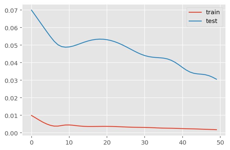

# Get the predicted values
predictions = model.predict(x_test)
predictions = scaler.inverse_transform(predictions)

1/3 [=========>....................] - ETA: 0s

3/3 [==============================] - ETA: 0s

3/3 [==============================] - 0s 31ms/step

y_test = y_test.reshape(-1,1)
y_test = scaler.inverse_transform(y_test)

# Calculate the mean absolute error (MAE)
mae = mean_absolute_error(y_test, predictions)
print('MAE: ' + str(round(mae, 1)))

# Calculate the root mean squarred error (RMSE)
rmse = np.sqrt(mean_squared_error(y_test,predictions))
print('RMSE: ' + str(round(rmse, 1)))

# Calculate the root mean squarred error (RMSE)
rmse = mean_squared_error(y_test, 
                          predictions,
                          squared = False)
print('RMSE: ' + str(round(rmse, 1)))

MAE: 1674.3
RMSE: 3525.8
RMSE: 3525.8

# Add the difference between the valid and predicted prices
train = data_Barcelona[:(len(x_train)+92)]
valid = data_Barcelona[(len(x_train)+91):]

valid.insert(1, "Predictions", predictions, True)
valid.insert(1, "Difference", valid["Predictions"] - valid["num_casos"], True)

# Zoom-in to a closer timeframe
# Date from which on the date is displayed
display_start_date = "2021-07-15" 
valid = valid[valid.index > display_start_date]
train = train[train.index > display_start_date]

# Visualize the data
matplotlib.style.use('ggplot')
fig, ax1 = plt.subplots(figsize=(22, 10), sharex=True)

# Data - Train
xt = train.index; 
yt = train[["num_casos"]]
# Data - Test / validation 
xv = valid.index; 
yv = valid[["num_casos", "Predictions"]]

# Plot
plt.title("Barcelona: Predictions vs Real infections", fontsize=20)
plt.ylabel("Nº Cases", fontsize=18)

plt.plot(yt, color="blue", linewidth=1.5)
plt.plot(yv["Predictions"], color="red", linewidth=1.5)
plt.plot(yv["num_casos"], color="green", linewidth=1.5)
plt.legend(["Train", "LSTM Predictions", "Test"], 
           loc="upper left", fontsize=18)

# Bar plot with the differences
x = valid.index
y = valid["Difference"]
plt.bar(x, y, width=0.2, color="grey")
plt.grid()
plt.show()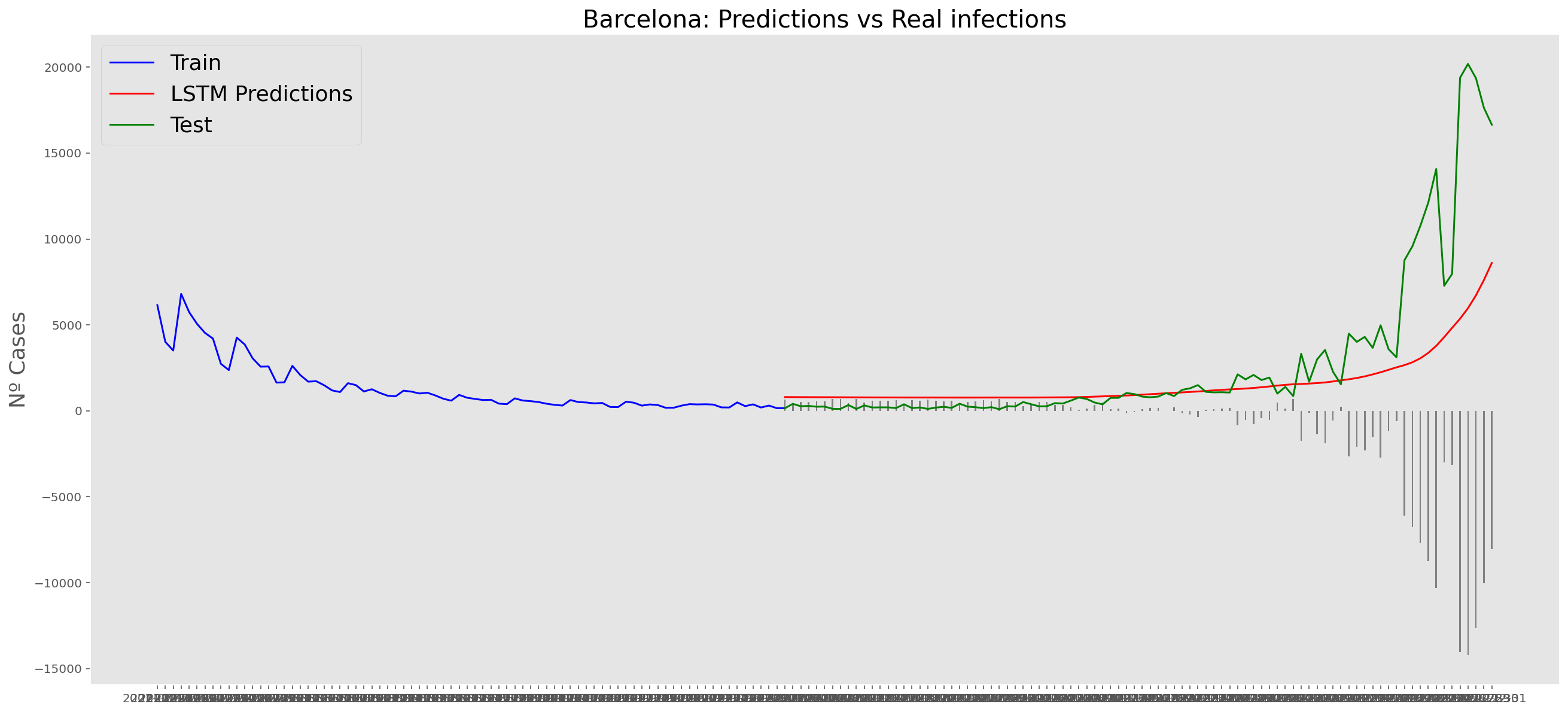

Madrid

data_Madrid = data_covid.loc[data_covid['provincia'] == 'Madrid']
data_Madrid = data_Madrid.set_index('fecha')
data_Madrid = data_Madrid.filter(['num_casos'])
data_Madrid = data_Madrid['2020-06-14':'2021-12-31']
data_Madrid

	num_casos
fecha
2020-06-14	81
2020-06-15	153
2020-06-16	91
2020-06-17	93
2020-06-18	85
...	...
2021-12-27	22958
2021-12-28	23811
2021-12-29	21914
2021-12-30	20666
2021-12-31	7556

566 rows × 1 columns

data_Madrid.describe()

	num_casos
count	566.000000
mean	1994.136042
std	2795.419848
min	28.000000
25%	550.250000
50%	1312.500000
75%	2282.500000
max	23811.000000

np_data_Madrid = data_Madrid.values

scaler = MinMaxScaler(feature_range=(0, 1))
scaled_data_Madrid = scaler.fit_transform(np_data_Madrid)
print(f'Longitud del conjunto de datos disponible: {len(scaled_data_Madrid)}')

Longitud del conjunto de datos disponible: 566

# Since we are going to predict future values based on the X past elements, 
# we need to create a list with those historic information for each element
historic_values = 90
scaled_data_Madrid_x = []
scaled_data_Madrid_y = []

for num_casos_i in range(historic_values, len(scaled_data_Madrid)):
    scaled_data_Madrid_x.append(scaled_data_Madrid[(num_casos_i-historic_values):num_casos_i, 0])
    scaled_data_Madrid_y.append(scaled_data_Madrid[num_casos_i, 0])

# Convert the x_train and y_train to numpy arrays
scaled_data_Madrid_x = np.array(scaled_data_Madrid_x)
scaled_data_Madrid_y = np.array(scaled_data_Madrid_y)

# Train data looks like
scaled_data_Madrid_x[235]

array([0.11428331, 0.14741622, 0.08796199, 0.06395324, 0.11087752,
       0.11272758, 0.08863474, 0.06862044, 0.09216667, 0.06046336,
       0.04620948, 0.08363117, 0.07660934, 0.06508851, 0.05621663,
       0.06428962, 0.04747088, 0.04288778, 0.06286003, 0.05844511,
       0.0505403 , 0.0445276 , 0.05243241, 0.04061725, 0.03943994,
       0.05398814, 0.05138124, 0.04734474, 0.04171047, 0.05159147,
       0.03830467, 0.03771602, 0.05474499, 0.05365177, 0.04726065,
       0.04360257, 0.05201194, 0.04036497, 0.03906151, 0.05360972,
       0.05096077, 0.05226422, 0.05625867, 0.04229912, 0.04974141,
       0.04700837, 0.07206828, 0.07745028, 0.06176681, 0.05815078,
       0.07400244, 0.05239036, 0.05247446, 0.07026027, 0.07009208,
       0.07698776, 0.05381996, 0.06079973, 0.07063869, 0.07370811,
       0.09796914, 0.09767481, 0.08493462, 0.08094017, 0.08867679,
       0.07139553, 0.05890762, 0.09666569, 0.09679183, 0.08846655,
       0.08459824, 0.09405878, 0.07101711, 0.0631964 , 0.092461  ,
       0.09771686, 0.08350502, 0.07568431, 0.08821427, 0.06386915,
       0.05398814, 0.08152882, 0.0865324 , 0.07240466, 0.06172476,
       0.07400244, 0.04566287, 0.04406509, 0.04633562, 0.06613968])

# Test data looks like
scaled_data_Madrid_y[235]

0.0639532439137199

# Since the first 90th values does not have historic, the dataset has been reduced in 90 values
print(f'Longitud datos de entrenamiento con historico: {len(scaled_data_Madrid_y)}')

Longitud datos de entrenamiento con historico: 476

# we split data in train and test
# as in previous analysis, we are going to predict a maximum of 91 days
x_train = scaled_data_Madrid_x[0:len(scaled_data_Madrid_x)-91]
y_train = scaled_data_Madrid_y[0:len(scaled_data_Madrid_y)-91]
print(f'Cantidad datos de entrenamiento: x={len(x_train)} - y={len(y_train)}')

x_test = scaled_data_Madrid_x[len(scaled_data_Madrid_x)-90:len(scaled_data_Madrid_x)]
y_test = scaled_data_Madrid_y[len(scaled_data_Madrid_y)-90:len(scaled_data_Madrid_y)]
print(f'Cantidad datos de test: x={len(x_test)} - y={len(y_test)}')

Cantidad datos de entrenamiento: x=385 - y=385
Cantidad datos de test: x=90 - y=90

# Reshape the data to feed de recurrent network
x_train = np.reshape(x_train, (x_train.shape[0], x_train.shape[1], 1))
print("Train data shape:")
print(x_train.shape)
print(y_train.shape)
x_test = np.reshape(x_test, (x_test.shape[0], x_test.shape[1], 1))
print("Test data shape:")
print(x_test.shape)
print(y_test.shape)

Train data shape:
(385, 90, 1)
(385,)
Test data shape:
(90, 90, 1)
(90,)

# Configure / setup the neural network model - LSTM
# Build the model
print('Build model...')
model = Sequential()
# Model with Neurons 
# Inputshape = neurons -> Timestamps
neurons= x_train.shape[1]
model.add(LSTM(90, 
               activation = 'relu',
               return_sequences = True, 
               input_shape = (x_train.shape[1], 1))) 
model.add(LSTM(50, 
               activation = 'relu',
               return_sequences = True)) 
model.add(LSTM(25, 
               activation = 'relu',
               return_sequences = False)) 
model.add(Dense(5, activation = 'relu'))
model.add(Dense(1))

Build model...

model.compile(optimizer='adam', loss='mean_squared_error')
model.summary()

Model: "sequential_7"

_________________________________________________________________

 Layer (type)                Output Shape              Param #

=================================================================

 lstm_21 (LSTM)              (None, 90, 90)            33120

 lstm_22 (LSTM)              (None, 90, 50)            28200

 lstm_23 (LSTM)              (None, 25)                7600

 dense_14 (Dense)            (None, 5)                 130

 dense_15 (Dense)            (None, 1)                 6

=================================================================

Total params: 69,056

Trainable params: 69,056

Non-trainable params: 0

_________________________________________________________________

# Training the model
# fit network
history = model.fit(x_train, 
                    y_train, 
                    batch_size = 1000, 
                    epochs = 50, 
                    validation_data = (x_test, y_test), 
                    verbose = 0)

plt.plot(history.history['loss'], label='train')
plt.plot(history.history['val_loss'], label='test')
plt.legend()
plt.show()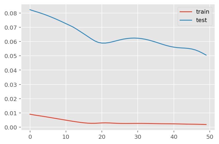

# Get the predicted values
predictions = model.predict(x_test)
predictions = scaler.inverse_transform(predictions)

1/3 [=========>....................] - ETA: 0s

3/3 [==============================] - ETA: 0s

3/3 [==============================] - 0s 31ms/step

y_test = y_test.reshape(-1,1)
y_test = scaler.inverse_transform(y_test)

# Calculate the mean absolute error (MAE)
mae = mean_absolute_error(y_test, predictions)
print('MAE: ' + str(round(mae, 1)))

# Calculate the root mean squarred error (RMSE)
rmse = np.sqrt(mean_squared_error(y_test,predictions))
print('RMSE: ' + str(round(rmse, 1)))

# Calculate the root mean squarred error (RMSE)
rmse = mean_squared_error(y_test, 
                          predictions,
                          squared = False)
print('RMSE: ' + str(round(rmse, 1)))

MAE: 2521.6
RMSE: 5345.2
RMSE: 5345.2

# Add the difference between the valid and predicted prices
train = data_Madrid[:(len(x_train)+92)]
valid = data_Madrid[(len(x_train)+91):]

valid.insert(1, "Predictions", predictions, True)
valid.insert(1, "Difference", valid["Predictions"] - valid["num_casos"], True)

# Zoom-in to a closer timeframe
# Date from which on the date is displayed
display_start_date = "2021-07-15" 
valid = valid[valid.index > display_start_date]
train = train[train.index > display_start_date]

# Visualize the data
matplotlib.style.use('ggplot')
fig, ax1 = plt.subplots(figsize=(22, 10), sharex=True)

# Data - Train
xt = train.index; 
yt = train[["num_casos"]]
# Data - Test / validation 
xv = valid.index; 
yv = valid[["num_casos", "Predictions"]]

# Plot
plt.title("Madrid: Predictions vs Real infections", fontsize=20)
plt.ylabel("Nº Cases", fontsize=18)

plt.plot(yt, color="blue", linewidth=1.5)
plt.plot(yv["Predictions"], color="red", linewidth=1.5)
plt.plot(yv["num_casos"], color="green", linewidth=1.5)
plt.legend(["Train", "LSTM Predictions", "Test"], 
           loc="upper left", fontsize=18)

# Bar plot with the differences
x = valid.index
y = valid["Difference"]
plt.bar(x, y, width=0.2, color="grey")
plt.grid()
plt.show()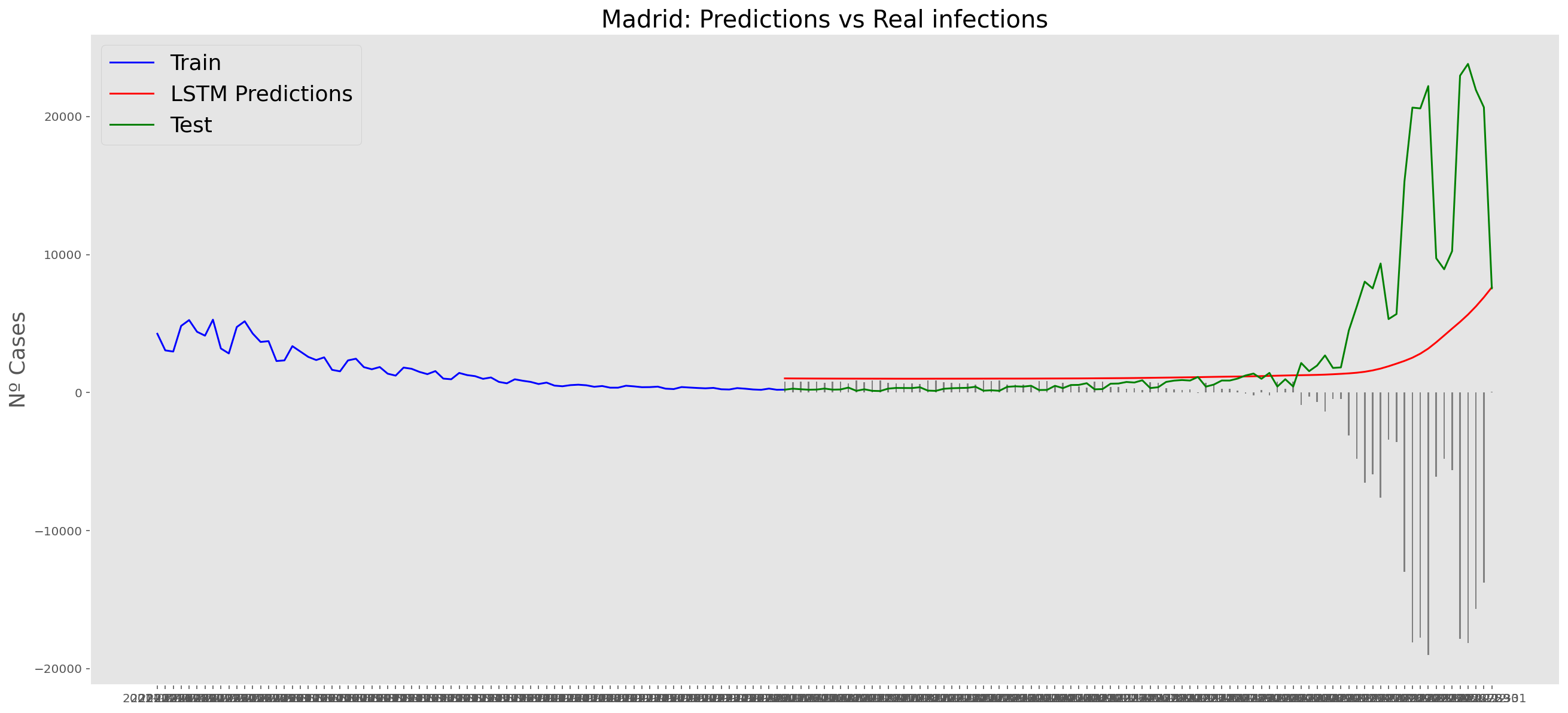

Malaga

data_Malaga = data_covid.loc[data_covid['provincia'] == 'Málaga']
data_Malaga = data_Malaga.set_index('fecha')
data_Malaga = data_Malaga.filter(['num_casos'])
data_Malaga = data_Malaga['2020-06-14':'2021-12-31']
data_Malaga

	num_casos
fecha
2020-06-14	2
2020-06-15	1
2020-06-16	1
2020-06-17	2
2020-06-18	2
...	...
2021-12-27	1627
2021-12-28	2772
2021-12-29	3080
2021-12-30	3075
2021-12-31	2646

566 rows × 1 columns

data_Malaga.describe()

	num_casos
count	566.000000
mean	339.227915
std	427.261346
min	1.000000
25%	110.000000
50%	193.500000
75%	344.750000
max	3080.000000

np_data_Malaga = data_Malaga.values

scaler = MinMaxScaler(feature_range=(0, 1))
scaled_data_Malaga = scaler.fit_transform(np_data_Malaga)
print(f'Longitud del conjunto de datos disponible: {len(scaled_data_Malaga)}')

Longitud del conjunto de datos disponible: 566

# Since we are going to predict future values based on the X past elements, 
# we need to create a list with those historic information for each element
historic_values = 90
scaled_data_Malaga_x = []
scaled_data_Malaga_y = []

for num_casos_i in range(historic_values, len(scaled_data_Malaga)):
    scaled_data_Malaga_x.append(scaled_data_Malaga[(num_casos_i-historic_values):num_casos_i, 0])
    scaled_data_Malaga_y.append(scaled_data_Malaga[num_casos_i, 0])

# Convert the x_train and y_train to numpy arrays
scaled_data_Malaga_x = np.array(scaled_data_Malaga_x)
scaled_data_Malaga_y = np.array(scaled_data_Malaga_y)

# Train data looks like
scaled_data_Malaga_x[235]

array([0.24423514, 0.21890224, 0.15621955, 0.12016889, 0.15329652,
       0.14420266, 0.14712569, 0.14647613, 0.11627152, 0.09418642,
       0.06722962, 0.09516077, 0.11042546, 0.06852874, 0.06950309,
       0.06658006, 0.04871712, 0.03442676, 0.05943488, 0.0490419 ,
       0.04936668, 0.04449497, 0.04157194, 0.03962325, 0.02923027,
       0.04157194, 0.04741799, 0.05131536, 0.04871712, 0.04287106,
       0.02760637, 0.02858071, 0.0422215 , 0.04092238, 0.03994804,
       0.03507632, 0.0506658 , 0.03020461, 0.02630724, 0.04092238,
       0.03117895, 0.04319584, 0.03702501, 0.0354011 , 0.02923027,
       0.02078597, 0.04157194, 0.04514453, 0.03832413, 0.04741799,
       0.0490419 , 0.0354011 , 0.02858071, 0.05326405, 0.05293927,
       0.05586229, 0.0422215 , 0.04027282, 0.03442676, 0.0490419 ,
       0.0659305 , 0.07794739, 0.0659305 , 0.05878532, 0.06203313,
       0.05034102, 0.03085417, 0.07047743, 0.05618707, 0.0776226 ,
       0.06138357, 0.07080221, 0.04124716, 0.04546931, 0.0659305 ,
       0.06690484, 0.05878532, 0.05488795, 0.05293927, 0.04352062,
       0.03637545, 0.0591101 , 0.06495615, 0.05975966, 0.05521273,
       0.05846054, 0.04481975, 0.04514453, 0.06235791, 0.07697304])

# Test data looks like
scaled_data_Malaga_y[235]

0.07340045469308218

# Since the first 90th values does not have historic, the dataset has been reduced in 90 values
print(f'Longitud datos de entrenamiento con historico: {len(scaled_data_Malaga_y)}')

Longitud datos de entrenamiento con historico: 476

# we split data in train and test
# as in previous analysis, we are going to predict a maximum of 91 days
x_train = scaled_data_Malaga_x[0:len(scaled_data_Malaga_x)-91]
y_train = scaled_data_Malaga_y[0:len(scaled_data_Malaga_y)-91]
print(f'Cantidad datos de entrenamiento: x={len(x_train)} - y={len(y_train)}')

x_test = scaled_data_Malaga_x[len(scaled_data_Malaga_x)-90:len(scaled_data_Malaga_x)]
y_test = scaled_data_Malaga_y[len(scaled_data_Malaga_y)-90:len(scaled_data_Malaga_y)]
print(f'Cantidad datos de test: x={len(x_test)} - y={len(y_test)}')

Cantidad datos de entrenamiento: x=385 - y=385
Cantidad datos de test: x=90 - y=90

# Reshape the data to feed de recurrent network
x_train = np.reshape(x_train, (x_train.shape[0], x_train.shape[1], 1))
print("Train data shape:")
print(x_train.shape)
print(y_train.shape)
x_test = np.reshape(x_test, (x_test.shape[0], x_test.shape[1], 1))
print("Test data shape:")
print(x_test.shape)
print(y_test.shape)

Train data shape:
(385, 90, 1)
(385,)
Test data shape:
(90, 90, 1)
(90,)

# Configure / setup the neural network model - LSTM
# Build the model
print('Build model...')
model = Sequential()
# Model with Neurons 
# Inputshape = neurons -> Timestamps
neurons= x_train.shape[1]
model.add(LSTM(90, 
               activation = 'relu',
               return_sequences = True, 
               input_shape = (x_train.shape[1], 1))) 
model.add(LSTM(50, 
               activation = 'relu',
               return_sequences = True)) 
model.add(LSTM(25, 
               activation = 'relu',
               return_sequences = False)) 
model.add(Dense(5, activation = 'relu'))
model.add(Dense(1))

Build model...

model.compile(optimizer='adam', loss='mean_squared_error')
model.summary()

Model: "sequential_8"

_________________________________________________________________

 Layer (type)                Output Shape              Param #

=================================================================

 lstm_24 (LSTM)              (None, 90, 90)            33120

 lstm_25 (LSTM)              (None, 90, 50)            28200

 lstm_26 (LSTM)              (None, 25)                7600

 dense_16 (Dense)            (None, 5)                 130

 dense_17 (Dense)            (None, 1)                 6

=================================================================

Total params: 69,056

Trainable params: 69,056

Non-trainable params: 0

_________________________________________________________________

# Training the model
# fit network
history = model.fit(x_train, 
                    y_train, 
                    batch_size = 1000, 
                    epochs = 50, 
                    validation_data = (x_test, y_test), 
                    verbose = 0)

plt.plot(history.history['loss'], label='train')
plt.plot(history.history['val_loss'], label='test')
plt.legend()
plt.show()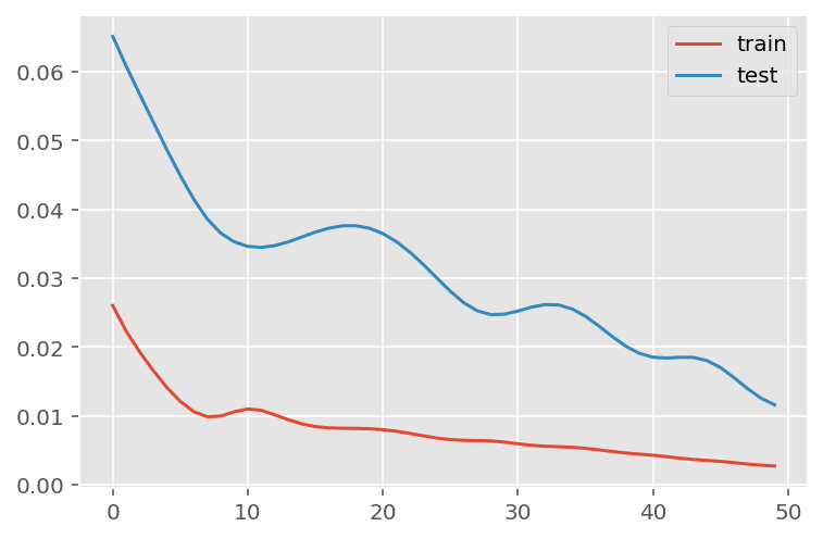

# Get the predicted values
predictions = model.predict(x_test)
predictions = scaler.inverse_transform(predictions)

1/3 [=========>....................] - ETA: 0s

3/3 [==============================] - ETA: 0s

3/3 [==============================] - 0s 31ms/step

y_test = y_test.reshape(-1,1)
y_test = scaler.inverse_transform(y_test)

# Calculate the mean absolute error (MAE)
mae = mean_absolute_error(y_test, predictions)
print('MAE: ' + str(round(mae, 1)))

# Calculate the root mean squarred error (RMSE)
rmse = np.sqrt(mean_squared_error(y_test,predictions))
print('RMSE: ' + str(round(rmse, 1)))

# Calculate the root mean squarred error (RMSE)
rmse = mean_squared_error(y_test, 
                          predictions,
                          squared = False)
print('RMSE: ' + str(round(rmse, 1)))

MAE: 197.7
RMSE: 331.7
RMSE: 331.7

# Add the difference between the valid and predicted prices
train = data_Malaga[:(len(x_train)+92)]
valid = data_Malaga[(len(x_train)+91):]

valid.insert(1, "Predictions", predictions, True)
valid.insert(1, "Difference", valid["Predictions"] - valid["num_casos"], True)

# Zoom-in to a closer timeframe
# Date from which on the date is displayed
display_start_date = "2021-07-15" 
valid = valid[valid.index > display_start_date]
train = train[train.index > display_start_date]

# Visualize the data
matplotlib.style.use('ggplot')
fig, ax1 = plt.subplots(figsize=(22, 10), sharex=True)

# Data - Train
xt = train.index; 
yt = train[["num_casos"]]
# Data - Test / validation 
xv = valid.index; 
yv = valid[["num_casos", "Predictions"]]

# Plot
plt.title("Malaga: Predictions vs Real infections", fontsize=20)
plt.ylabel("Nº Cases", fontsize=18)

plt.plot(yt, color="blue", linewidth=1.5)
plt.plot(yv["Predictions"], color="red", linewidth=1.5)
plt.plot(yv["num_casos"], color="green", linewidth=1.5)
plt.legend(["Train", "LSTM Predictions", "Test"], 
           loc="upper left", fontsize=18)

# Bar plot with the differences
x = valid.index
y = valid["Difference"]
plt.bar(x, y, width=0.2, color="grey")
plt.grid()
plt.show()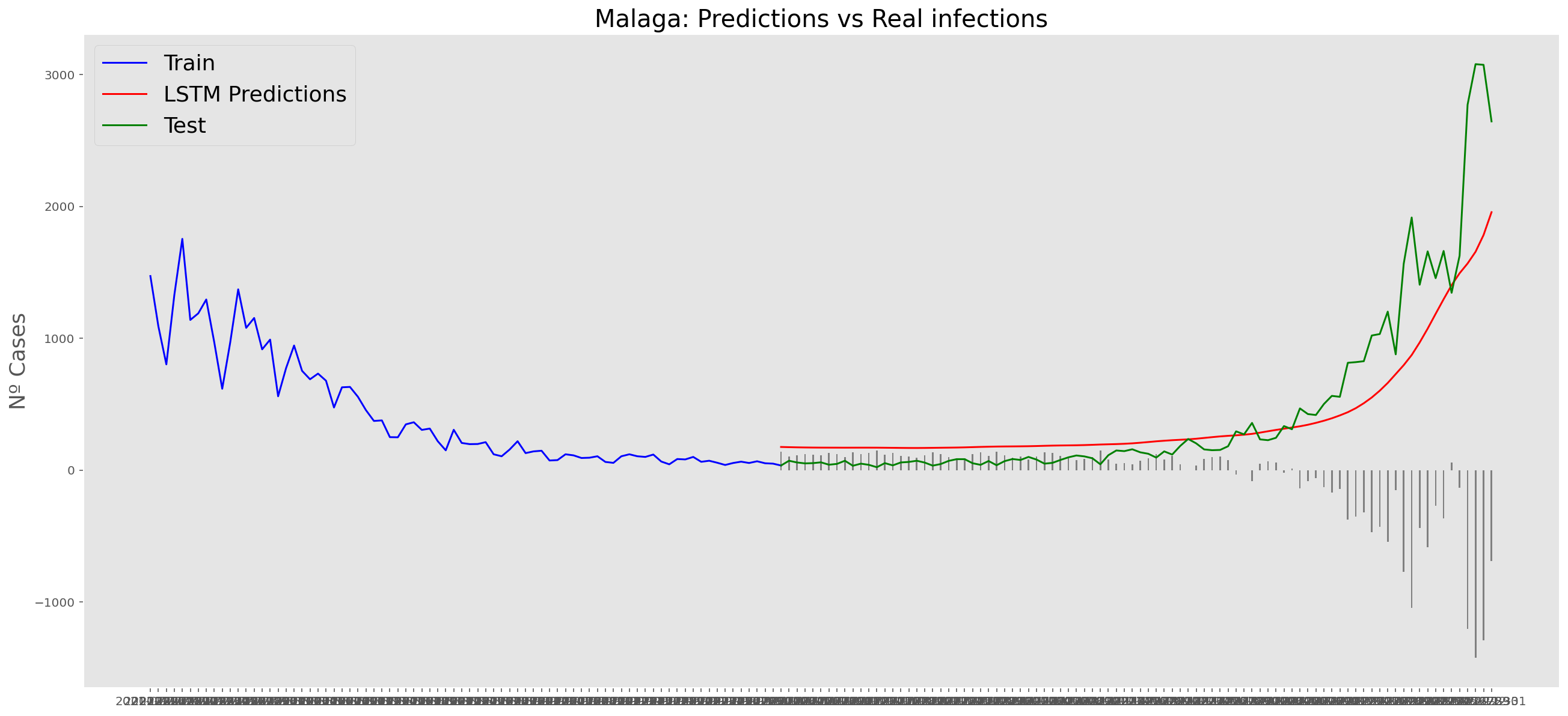

Sevilla

data_Sevilla = data_covid.loc[data_covid['provincia'] == 'Sevilla']
data_Sevilla = data_Sevilla.set_index('fecha')
data_Sevilla = data_Sevilla.filter(['num_casos'])
data_Sevilla = data_Sevilla['2020-06-14':'2021-12-31']
data_Sevilla

	num_casos
fecha
2020-06-14	0
2020-06-15	2
2020-06-16	1
2020-06-17	0
2020-06-18	0
...	...
2021-12-27	2617
2021-12-28	3190
2021-12-29	3692
2021-12-30	3508
2021-12-31	2816

566 rows × 1 columns

data_Sevilla.describe()

	num_casos
count	566.000000
mean	383.807420
std	454.714408
min	0.000000
25%	112.750000
50%	260.500000
75%	459.000000
max	3692.000000

np_data_Sevilla = data_Sevilla.values

scaler = MinMaxScaler(feature_range=(0, 1))
scaled_data_Sevilla = scaler.fit_transform(np_data_Sevilla)
print(f'Longitud del conjunto de datos disponible: {len(scaled_data_Sevilla)}')

Longitud del conjunto de datos disponible: 566

# Since we are going to predict future values based on the X past elements, 
# we need to create a list with those historic information for each element
historic_values = 90
scaled_data_Sevilla_x = []
scaled_data_Sevilla_y = []

for num_casos_i in range(historic_values, len(scaled_data_Sevilla)):
    scaled_data_Sevilla_x.append(scaled_data_Sevilla[(num_casos_i-historic_values):num_casos_i, 0])
    scaled_data_Sevilla_y.append(scaled_data_Sevilla[num_casos_i, 0])

# Convert the x_train and y_train to numpy arrays
scaled_data_Sevilla_x = np.array(scaled_data_Sevilla_x)
scaled_data_Sevilla_y = np.array(scaled_data_Sevilla_y)

# Train data looks like
scaled_data_Sevilla_x[235]

array([0.18634886, 0.19799567, 0.14626219, 0.0896533 , 0.13894908,
       0.1695558 , 0.14572048, 0.12242687, 0.13434453, 0.06500542,
       0.05390033, 0.08206934, 0.08667389, 0.09452871, 0.06798483,
       0.05904659, 0.04252438, 0.0343987 , 0.06554713, 0.06473456,
       0.05444204, 0.0503792 , 0.05796316, 0.04577465, 0.03819068,
       0.04712893, 0.0528169 , 0.0663597 , 0.06013001, 0.05119177,
       0.03764897, 0.031961  , 0.05119177, 0.05010834, 0.04739978,
       0.05119177, 0.05390033, 0.03927411, 0.03737811, 0.06013001,
       0.05633803, 0.05606717, 0.05850488, 0.06473456, 0.04658722,
       0.04198267, 0.07150596, 0.07340195, 0.05823402, 0.08071506,
       0.07773564, 0.05877573, 0.05471289, 0.07990249, 0.08829902,
       0.0872156 , 0.09019502, 0.07069339, 0.08775731, 0.08396533,
       0.14951246, 0.12432286, 0.12269772, 0.12378115, 0.13028169,
       0.11348862, 0.07936078, 0.13299025, 0.12269772, 0.11213434,
       0.12107259, 0.12432286, 0.09723727, 0.07042254, 0.09886241,
       0.11782232, 0.10157096, 0.10346696, 0.12621885, 0.08342362,
       0.07340195, 0.0847779 , 0.08559047, 0.11159263, 0.10292524,
       0.08911159, 0.07502709, 0.04821235, 0.08315276, 0.09913326])

# Test data looks like
scaled_data_Sevilla_y[235]

0.10861321776814734

# Since the first 90th values does not have historic, the dataset has been reduced in 90 values
print(f'Longitud datos de entrenamiento con historico: {len(scaled_data_Sevilla_y)}')

Longitud datos de entrenamiento con historico: 476

# we split data in train and test
# as in previous analysis, we are going to predict a maximum of 91 days
x_train = scaled_data_Sevilla_x[0:len(scaled_data_Sevilla_x)-91]
y_train = scaled_data_Sevilla_y[0:len(scaled_data_Sevilla_y)-91]
print(f'Cantidad datos de entrenamiento: x={len(x_train)} - y={len(y_train)}')

x_test = scaled_data_Sevilla_x[len(scaled_data_Sevilla_x)-90:len(scaled_data_Sevilla_x)]
y_test = scaled_data_Sevilla_y[len(scaled_data_Sevilla_y)-90:len(scaled_data_Sevilla_y)]
print(f'Cantidad datos de test: x={len(x_test)} - y={len(y_test)}')

Cantidad datos de entrenamiento: x=385 - y=385
Cantidad datos de test: x=90 - y=90

# Reshape the data to feed de recurrent network
x_train = np.reshape(x_train, (x_train.shape[0], x_train.shape[1], 1))
print("Train data shape:")
print(x_train.shape)
print(y_train.shape)
x_test = np.reshape(x_test, (x_test.shape[0], x_test.shape[1], 1))
print("Test data shape:")
print(x_test.shape)
print(y_test.shape)

Train data shape:
(385, 90, 1)
(385,)
Test data shape:
(90, 90, 1)
(90,)

# Configure / setup the neural network model - LSTM
# Build the model
print('Build model...')
model = Sequential()
# Model with Neurons 
# Inputshape = neurons -> Timestamps
neurons= x_train.shape[1]
model.add(LSTM(90, 
               activation = 'relu',
               return_sequences = True, 
               input_shape = (x_train.shape[1], 1))) 
model.add(LSTM(50, 
               activation = 'relu',
               return_sequences = True)) 
model.add(LSTM(25, 
               activation = 'relu',
               return_sequences = False)) 
model.add(Dense(5, activation = 'relu'))
model.add(Dense(1))

Build model...

model.compile(optimizer='adam', loss='mean_squared_error')
model.summary()

Model: "sequential_9"

_________________________________________________________________

 Layer (type)                Output Shape              Param #

=================================================================

 lstm_27 (LSTM)              (None, 90, 90)            33120

 lstm_28 (LSTM)              (None, 90, 50)            28200

 lstm_29 (LSTM)              (None, 25)                7600

 dense_18 (Dense)            (None, 5)                 130

 dense_19 (Dense)            (None, 1)                 6

=================================================================

Total params: 69,056

Trainable params: 69,056

Non-trainable params: 0

_________________________________________________________________

# Training the model
# fit network
history = model.fit(x_train, 
                    y_train, 
                    batch_size = 1000, 
                    epochs = 50, 
                    validation_data = (x_test, y_test), 
                    verbose = 0)

plt.plot(history.history['loss'], label='train')
plt.plot(history.history['val_loss'], label='test')
plt.legend()
plt.show()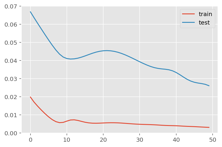

# Get the predicted values
predictions = model.predict(x_test)
predictions = scaler.inverse_transform(predictions)

1/3 [=========>....................] - ETA: 0s

3/3 [==============================] - ETA: 0s

3/3 [==============================] - 0s 32ms/step

y_test = y_test.reshape(-1,1)
y_test = scaler.inverse_transform(y_test)

# Calculate the mean absolute error (MAE)
mae = mean_absolute_error(y_test, predictions)
print('MAE: ' + str(round(mae, 1)))

# Calculate the root mean squarred error (RMSE)
rmse = np.sqrt(mean_squared_error(y_test,predictions))
print('RMSE: ' + str(round(rmse, 1)))

# Calculate the root mean squarred error (RMSE)
rmse = mean_squared_error(y_test, 
                          predictions,
                          squared = False)
print('RMSE: ' + str(round(rmse, 1)))

MAE: 329.2
RMSE: 595.9
RMSE: 595.9

# Add the difference between the valid and predicted prices
train = data_Sevilla[:(len(x_train)+92)]
valid = data_Sevilla[(len(x_train)+91):]

valid.insert(1, "Predictions", predictions, True)
valid.insert(1, "Difference", valid["Predictions"] - valid["num_casos"], True)

# Zoom-in to a closer timeframe
# Date from which on the date is displayed
display_start_date = "2021-07-15" 
valid = valid[valid.index > display_start_date]
train = train[train.index > display_start_date]

# Visualize the data
matplotlib.style.use('ggplot')
fig, ax1 = plt.subplots(figsize=(22, 10), sharex=True)

# Data - Train
xt = train.index; 
yt = train[["num_casos"]]
# Data - Test / validation 
xv = valid.index; 
yv = valid[["num_casos", "Predictions"]]

# Plot
plt.title("Sevilla: Predictions vs Real infections", fontsize=20)
plt.ylabel("Nº Cases", fontsize=18)

plt.plot(yt, color="blue", linewidth=1.5)
plt.plot(yv["Predictions"], color="red", linewidth=1.5)
plt.plot(yv["num_casos"], color="green", linewidth=1.5)
plt.legend(["Train", "LSTM Predictions", "Test"], 
           loc="upper left", fontsize=18)

# Bar plot with the differences
x = valid.index
y = valid["Difference"]
plt.bar(x, y, width=0.2, color="grey")
plt.grid()
plt.show()