As previously mentioned, the visual analysis will focus on the following provinces:
Asturias
Barcelona
Madrid
Málaga
Sevilla
First, we need to load packages and clean data generated during previous tasks:
pacman::p_load( here, # file locator tidyverse, # data management and ggplot2 graphics skimr, # get overview of data janitor, # produce and adorn tabulations and cross-tabulations lubridate, # manage dates PerformanceAnalytics, factoextra, tsibble, ggfortify)hosp_data <-readRDS(here("data", "clean", "final_hosp_data.rds"))hosp_data
# A tibble: 122,850 × 8
   provincia sexo  grupo_edad fecha      num_casos num_hosp num_uci num_def
   <chr>     <chr> <chr>      <date>         <dbl>    <dbl>   <dbl>   <dbl>
 1 Barcelona H     0-9        2020-01-01         0        0       0       0
 2 Barcelona H     10-19      2020-01-01         0        0       0       0
 3 Barcelona H     20-29      2020-01-01         0        0       0       0
 4 Barcelona H     30-39      2020-01-01         0        0       0       0
 5 Barcelona H     40-49      2020-01-01         0        0       0       0
 6 Barcelona H     50-59      2020-01-01         0        0       0       0
 7 Barcelona H     60-69      2020-01-01         0        0       0       0
 8 Barcelona H     70-79      2020-01-01         0        0       0       0
 9 Barcelona H     80+        2020-01-01         0        0       0       0
10 Barcelona H     NC         2020-01-01         0        0       0       0
# … with 122,840 more rows
Asturias
data_asturias <- hosp_data %>%filter(provincia =="Asturias") %>%select(-provincia) %>%as_tsibble(index = fecha, key =c(sexo, grupo_edad)) %>%mutate(ola =case_when( fecha <as.Date("2020-06-21", format ="%Y-%m-%d") ~"1_ola", fecha <as.Date("2020-12-06", format ="%Y-%m-%d") ~"2_ola", fecha <as.Date("2021-03-14", format ="%Y-%m-%d") ~"3_ola", fecha <as.Date("2021-06-19", format ="%Y-%m-%d") ~"4_ola", fecha <as.Date("2021-10-13", format ="%Y-%m-%d") ~"5_ola",TRUE~"6_ola", ))data_asturias
# A tsibble: 24,570 x 8 [1D]
# Key:       sexo, grupo_edad [30]
   sexo  grupo_edad fecha      num_casos num_hosp num_uci num_def ola
   <chr> <chr>      <date>         <dbl>    <dbl>   <dbl>   <dbl> <chr>
 1 H     0-9        2020-01-01         0        0       0       0 1_ola
 2 H     0-9        2020-01-02         0        0       0       0 1_ola
 3 H     0-9        2020-01-03         0        0       0       0 1_ola
 4 H     0-9        2020-01-04         0        0       0       0 1_ola
 5 H     0-9        2020-01-05         0        0       0       0 1_ola
 6 H     0-9        2020-01-06         0        0       0       0 1_ola
 7 H     0-9        2020-01-07         0        0       0       0 1_ola
 8 H     0-9        2020-01-08         0        0       0       0 1_ola
 9 H     0-9        2020-01-09         0        0       0       0 1_ola
10 H     0-9        2020-01-10         0        0       0       0 1_ola
# … with 24,560 more rows
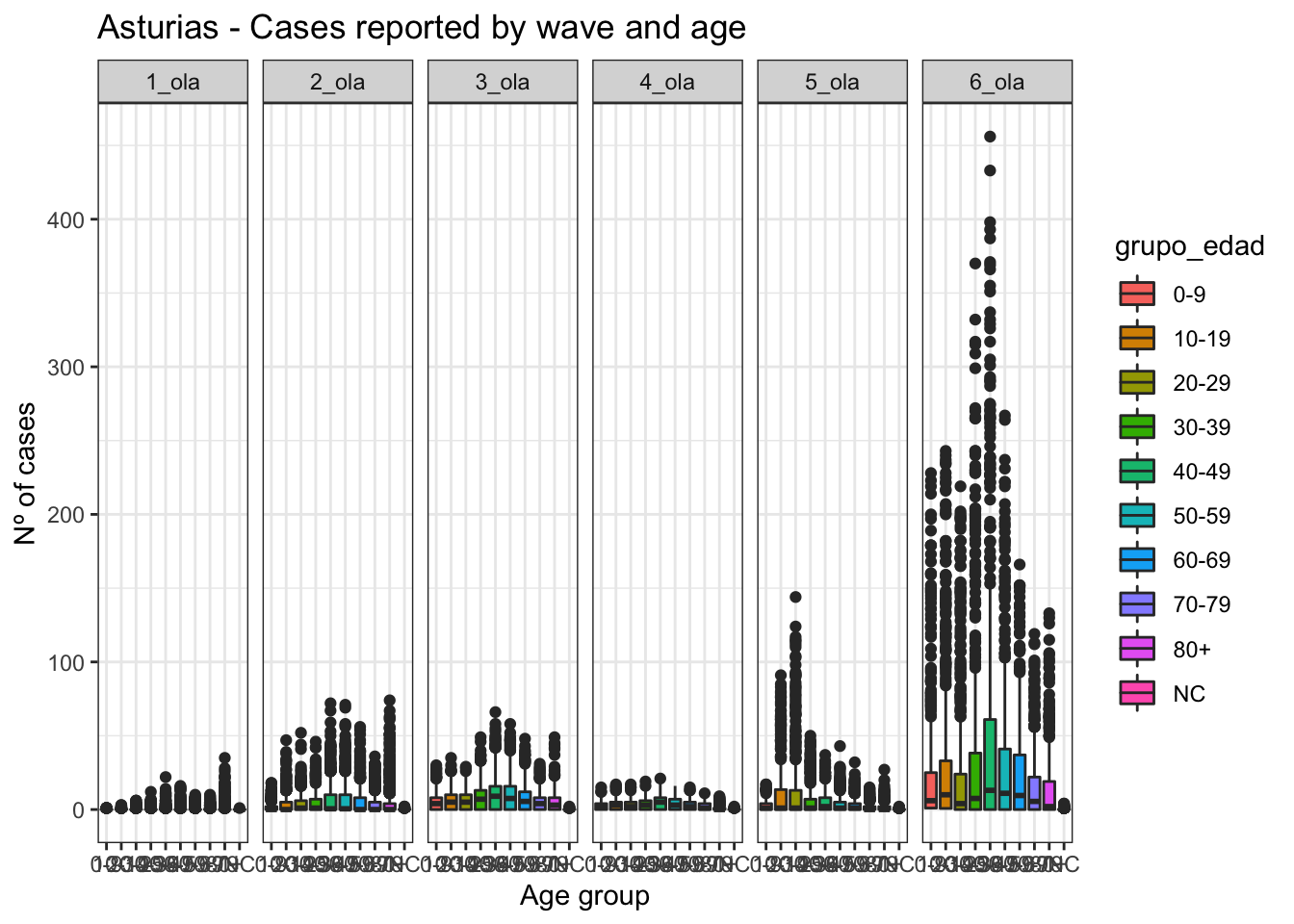
by wave
data_asturias %>%ggplot(aes(x=grupo_edad, y=num_casos)) +geom_boxplot(aes(fill=grupo_edad)) +facet_grid(. ~ ola) +theme(legend.position ="top") +labs(title="Asturias - Cases reported by wave and age",x ="Age group", y ="Nº of cases") +theme_bw()
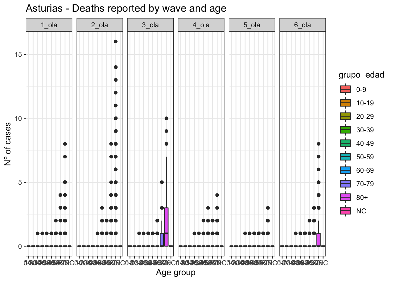
data_asturias %>%ggplot(aes(x=grupo_edad, y=num_def)) +geom_boxplot(aes(fill=grupo_edad)) +facet_grid(. ~ ola) +theme(legend.position ="top") +labs(title="Asturias - Deaths reported by wave and age",x ="Age group", y ="Nº of cases") +theme_bw()
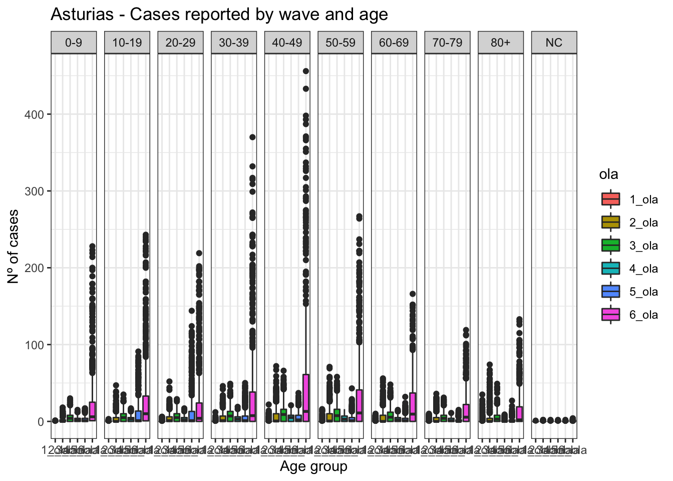
by age group
data_asturias %>%ggplot(aes(x=ola, y=num_casos)) +geom_boxplot(aes(fill=ola)) +facet_grid(. ~ grupo_edad) +theme(legend.position ="top") +labs(title="Asturias - Cases reported by wave and age",x ="Age group", y ="Nº of cases") +theme_bw()
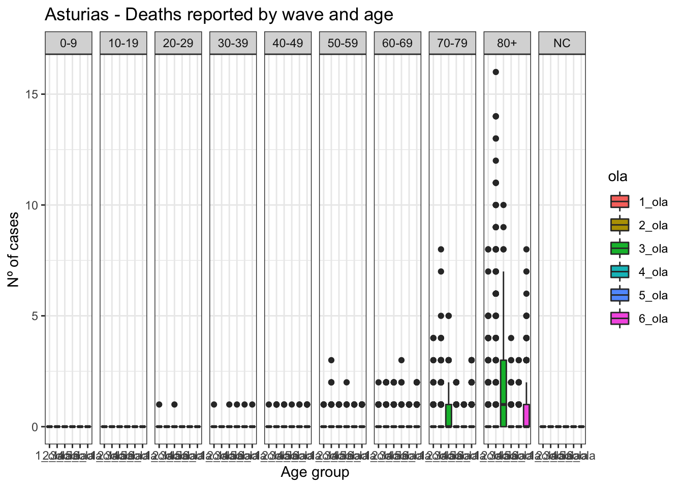
data_asturias %>%ggplot(aes(x=ola, y=num_def)) +geom_boxplot(aes(fill=ola)) +facet_grid(. ~ grupo_edad) +theme(legend.position ="top") +labs(title="Asturias - Deaths reported by wave and age",x ="Age group", y ="Nº of cases") +theme_bw()
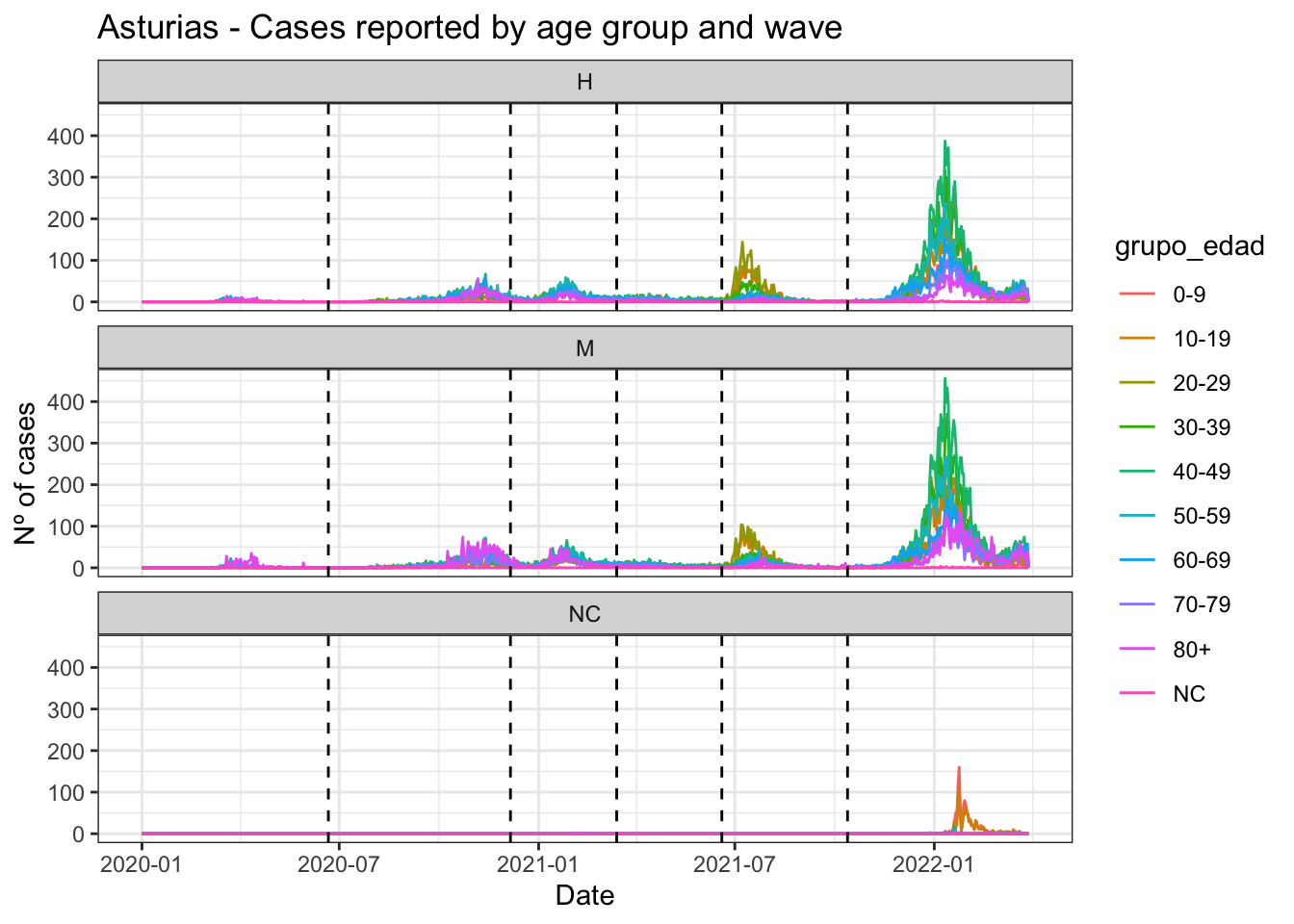
data_asturias %>%ggplot(aes(x=fecha, y=num_casos)) +geom_line(aes(color=grupo_edad)) +geom_vline(xintercept =as.Date("2020-06-21", format ="%Y-%m-%d"), linetype="dashed") +geom_vline(xintercept =as.Date("2020-12-06", format ="%Y-%m-%d"), linetype="dashed") +geom_vline(xintercept =as.Date("2021-03-14", format ="%Y-%m-%d"), linetype="dashed") +geom_vline(xintercept =as.Date("2021-06-19", format ="%Y-%m-%d"), linetype="dashed") +geom_vline(xintercept =as.Date("2021-10-13", format ="%Y-%m-%d"), linetype="dashed") +facet_wrap(~sexo, ncol=1) +theme(legend.position ="top") +labs(title="Asturias - Cases reported by age group and wave",x ="Date", y ="Nº of cases") +theme_bw()
by sex
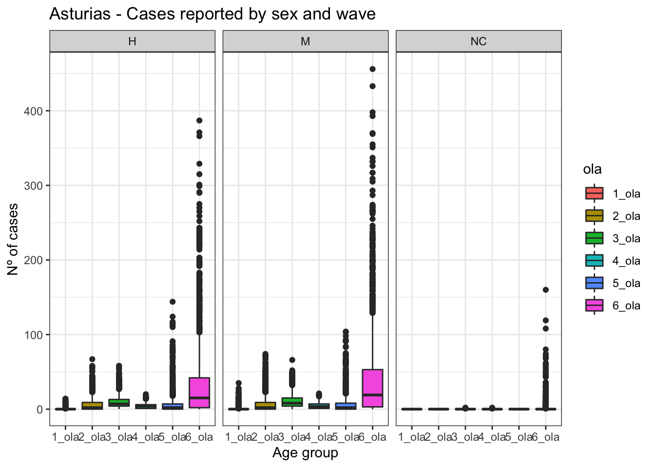
data_asturias %>%ggplot(aes(x=ola, y=num_casos)) +geom_boxplot(aes(fill=ola)) +facet_grid(. ~ sexo) +theme(legend.position ="top") +labs(title="Asturias - Cases reported by sex and wave",x ="Age group", y ="Nº of cases") +theme_bw()
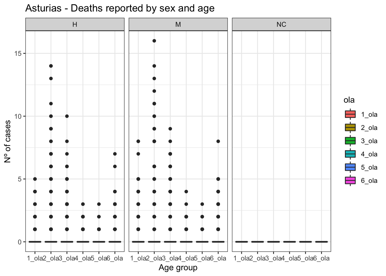
data_asturias %>%ggplot(aes(x=ola, y=num_def)) +geom_boxplot(aes(fill=ola)) +facet_grid(. ~ sexo) +theme(legend.position ="top") +labs(title="Asturias - Deaths reported by sex and age",x ="Age group", y ="Nº of cases") +theme_bw()
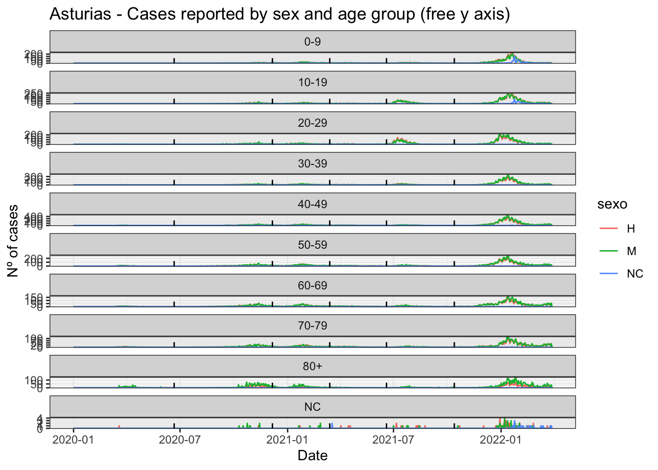
data_asturias %>%ggplot(aes(x=fecha, y=num_casos)) +geom_line(aes(color=sexo)) +geom_vline(xintercept =as.Date("2020-06-21", format ="%Y-%m-%d"), linetype="dashed") +geom_vline(xintercept =as.Date("2020-12-06", format ="%Y-%m-%d"), linetype="dashed") +geom_vline(xintercept =as.Date("2021-03-14", format ="%Y-%m-%d"), linetype="dashed") +geom_vline(xintercept =as.Date("2021-06-19", format ="%Y-%m-%d"), linetype="dashed") +geom_vline(xintercept =as.Date("2021-10-13", format ="%Y-%m-%d"), linetype="dashed") +facet_wrap(~grupo_edad, scales ="free_y", ncol=1) +theme(legend.position ="top") +labs(title="Asturias - Cases reported by sex and age group (free y axis)",x ="Date", y ="Nº of cases") +theme_bw()
Barcelona
data_Barcelona <- hosp_data %>%filter(provincia =="Barcelona") %>%select(-provincia) %>%as_tsibble(index = fecha, key =c(sexo, grupo_edad)) %>%mutate(ola =case_when( fecha <as.Date("2020-06-21", format ="%Y-%m-%d") ~"1_ola", fecha <as.Date("2020-12-06", format ="%Y-%m-%d") ~"2_ola", fecha <as.Date("2021-03-14", format ="%Y-%m-%d") ~"3_ola", fecha <as.Date("2021-06-19", format ="%Y-%m-%d") ~"4_ola", fecha <as.Date("2021-10-13", format ="%Y-%m-%d") ~"5_ola",TRUE~"6_ola", ))data_Barcelona
# A tsibble: 24,570 x 8 [1D]
# Key:       sexo, grupo_edad [30]
   sexo  grupo_edad fecha      num_casos num_hosp num_uci num_def ola
   <chr> <chr>      <date>         <dbl>    <dbl>   <dbl>   <dbl> <chr>
 1 H     0-9        2020-01-01         0        0       0       0 1_ola
 2 H     0-9        2020-01-02         0        0       0       0 1_ola
 3 H     0-9        2020-01-03         0        0       0       0 1_ola
 4 H     0-9        2020-01-04         0        0       0       0 1_ola
 5 H     0-9        2020-01-05         0        0       0       0 1_ola
 6 H     0-9        2020-01-06         0        0       0       0 1_ola
 7 H     0-9        2020-01-07         0        0       0       0 1_ola
 8 H     0-9        2020-01-08         0        0       0       0 1_ola
 9 H     0-9        2020-01-09         0        0       0       0 1_ola
10 H     0-9        2020-01-10         1        0       0       0 1_ola
# … with 24,560 more rows
by wave
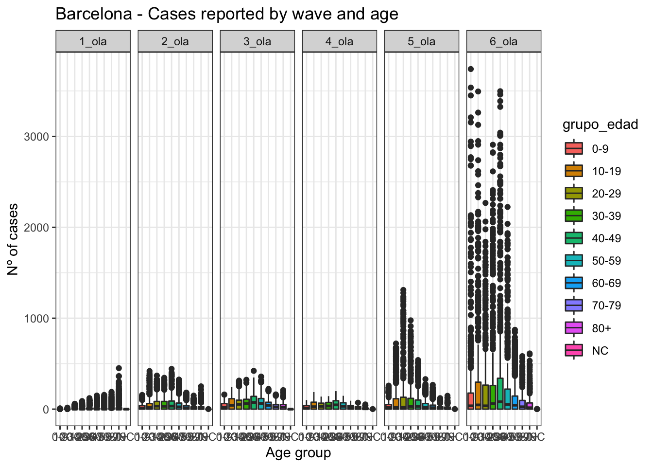
data_Barcelona %>%ggplot(aes(x=grupo_edad, y=num_casos)) +geom_boxplot(aes(fill=grupo_edad)) +facet_grid(. ~ ola) +theme(legend.position ="top") +labs(title="Barcelona - Cases reported by wave and age",x ="Age group", y ="Nº of cases") +theme_bw()
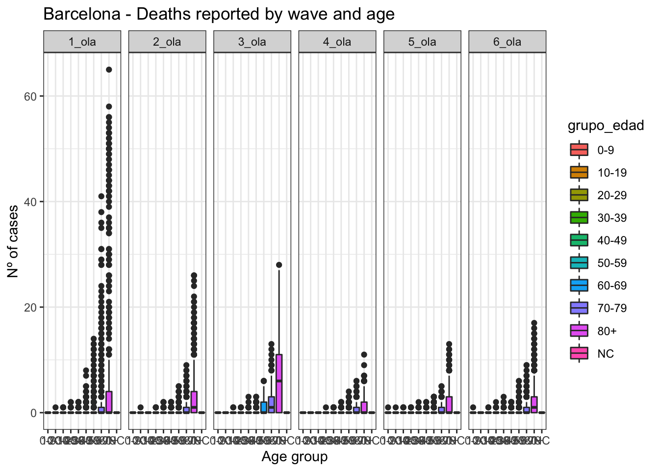
data_Barcelona %>%ggplot(aes(x=grupo_edad, y=num_def)) +geom_boxplot(aes(fill=grupo_edad)) +facet_grid(. ~ ola) +theme(legend.position ="top") +labs(title="Barcelona - Deaths reported by wave and age",x ="Age group", y ="Nº of cases") +theme_bw()
by age group
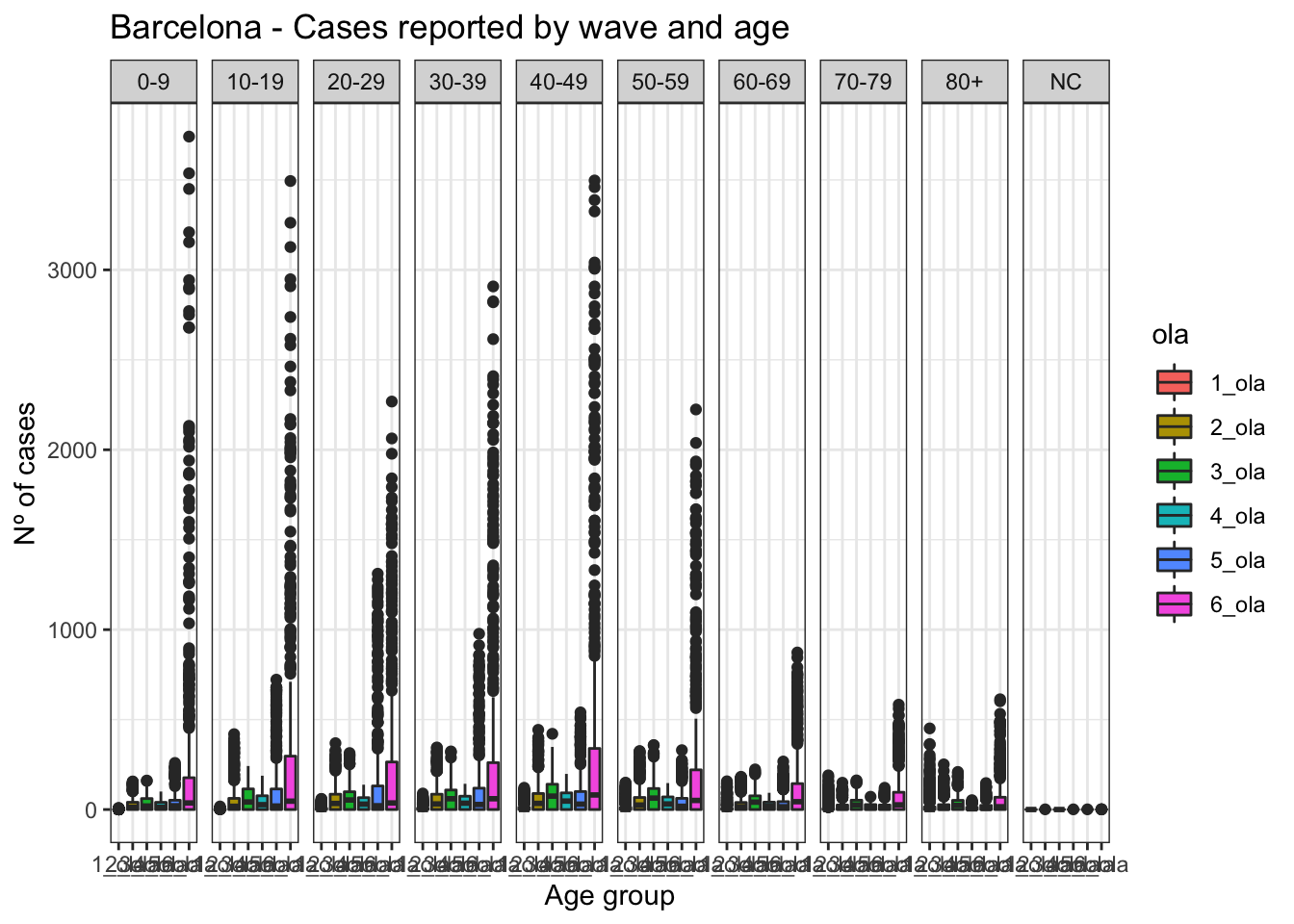
data_Barcelona %>%ggplot(aes(x=ola, y=num_casos)) +geom_boxplot(aes(fill=ola)) +facet_grid(. ~ grupo_edad) +theme(legend.position ="top") +labs(title="Barcelona - Cases reported by wave and age",x ="Age group", y ="Nº of cases") +theme_bw()
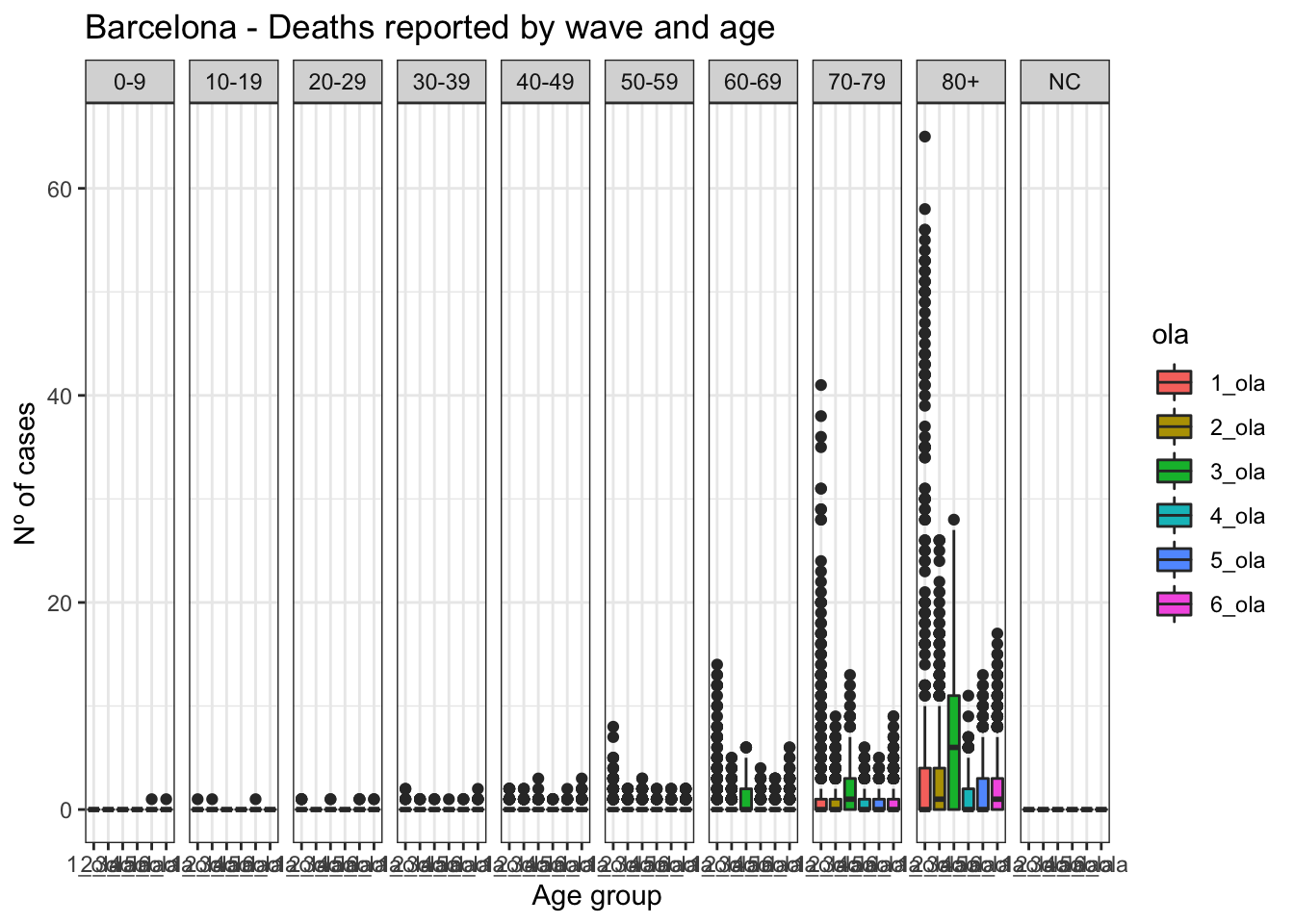
data_Barcelona %>%ggplot(aes(x=ola, y=num_def)) +geom_boxplot(aes(fill=ola)) +facet_grid(. ~ grupo_edad) +theme(legend.position ="top") +labs(title="Barcelona - Deaths reported by wave and age",x ="Age group", y ="Nº of cases") +theme_bw()
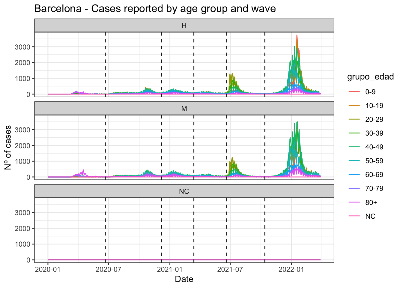
data_Barcelona %>%ggplot(aes(x=fecha, y=num_casos)) +geom_line(aes(color=grupo_edad)) +geom_vline(xintercept =as.Date("2020-06-21", format ="%Y-%m-%d"), linetype="dashed") +geom_vline(xintercept =as.Date("2020-12-06", format ="%Y-%m-%d"), linetype="dashed") +geom_vline(xintercept =as.Date("2021-03-14", format ="%Y-%m-%d"), linetype="dashed") +geom_vline(xintercept =as.Date("2021-06-19", format ="%Y-%m-%d"), linetype="dashed") +geom_vline(xintercept =as.Date("2021-10-13", format ="%Y-%m-%d"), linetype="dashed") +facet_wrap(~sexo, ncol=1) +theme(legend.position ="top") +labs(title="Barcelona - Cases reported by age group and wave",x ="Date", y ="Nº of cases") +theme_bw()
by sex
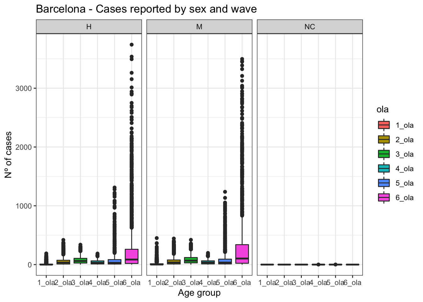
data_Barcelona %>%ggplot(aes(x=ola, y=num_casos)) +geom_boxplot(aes(fill=ola)) +facet_grid(. ~ sexo) +theme(legend.position ="top") +labs(title="Barcelona - Cases reported by sex and wave",x ="Age group", y ="Nº of cases") +theme_bw()
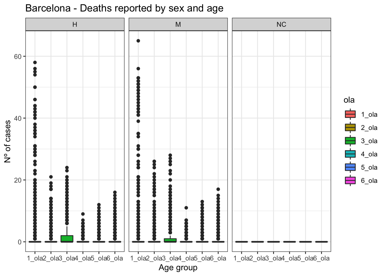
data_Barcelona %>%ggplot(aes(x=ola, y=num_def)) +geom_boxplot(aes(fill=ola)) +facet_grid(. ~ sexo) +theme(legend.position ="top") +labs(title="Barcelona - Deaths reported by sex and age",x ="Age group", y ="Nº of cases") +theme_bw()
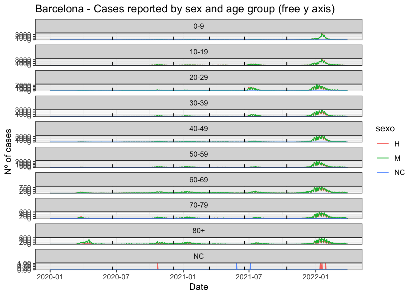
data_Barcelona %>%ggplot(aes(x=fecha, y=num_casos)) +geom_line(aes(color=sexo)) +geom_vline(xintercept =as.Date("2020-06-21", format ="%Y-%m-%d"), linetype="dashed") +geom_vline(xintercept =as.Date("2020-12-06", format ="%Y-%m-%d"), linetype="dashed") +geom_vline(xintercept =as.Date("2021-03-14", format ="%Y-%m-%d"), linetype="dashed") +geom_vline(xintercept =as.Date("2021-06-19", format ="%Y-%m-%d"), linetype="dashed") +geom_vline(xintercept =as.Date("2021-10-13", format ="%Y-%m-%d"), linetype="dashed") +facet_wrap(~grupo_edad, scales ="free_y", ncol=1) +theme(legend.position ="top") +labs(title="Barcelona - Cases reported by sex and age group (free y axis)",x ="Date", y ="Nº of cases") +theme_bw()
Madrid
data_Madrid <- hosp_data %>%filter(provincia =="Madrid") %>%select(-provincia) %>%as_tsibble(index = fecha, key =c(sexo, grupo_edad)) %>%mutate(ola =case_when( fecha <as.Date("2020-06-21", format ="%Y-%m-%d") ~"1_ola", fecha <as.Date("2020-12-06", format ="%Y-%m-%d") ~"2_ola", fecha <as.Date("2021-03-14", format ="%Y-%m-%d") ~"3_ola", fecha <as.Date("2021-06-19", format ="%Y-%m-%d") ~"4_ola", fecha <as.Date("2021-10-13", format ="%Y-%m-%d") ~"5_ola",TRUE~"6_ola", ))data_Madrid
# A tsibble: 24,570 x 8 [1D]
# Key:       sexo, grupo_edad [30]
   sexo  grupo_edad fecha      num_casos num_hosp num_uci num_def ola
   <chr> <chr>      <date>         <dbl>    <dbl>   <dbl>   <dbl> <chr>
 1 H     0-9        2020-01-01         0        0       0       0 1_ola
 2 H     0-9        2020-01-02         0        1       1       0 1_ola
 3 H     0-9        2020-01-03         0        0       0       0 1_ola
 4 H     0-9        2020-01-04         0        0       0       0 1_ola
 5 H     0-9        2020-01-05         0        0       0       0 1_ola
 6 H     0-9        2020-01-06         0        0       0       0 1_ola
 7 H     0-9        2020-01-07         0        0       0       0 1_ola
 8 H     0-9        2020-01-08         0        0       0       0 1_ola
 9 H     0-9        2020-01-09         0        0       0       0 1_ola
10 H     0-9        2020-01-10         0        0       0       0 1_ola
# … with 24,560 more rows
by wave
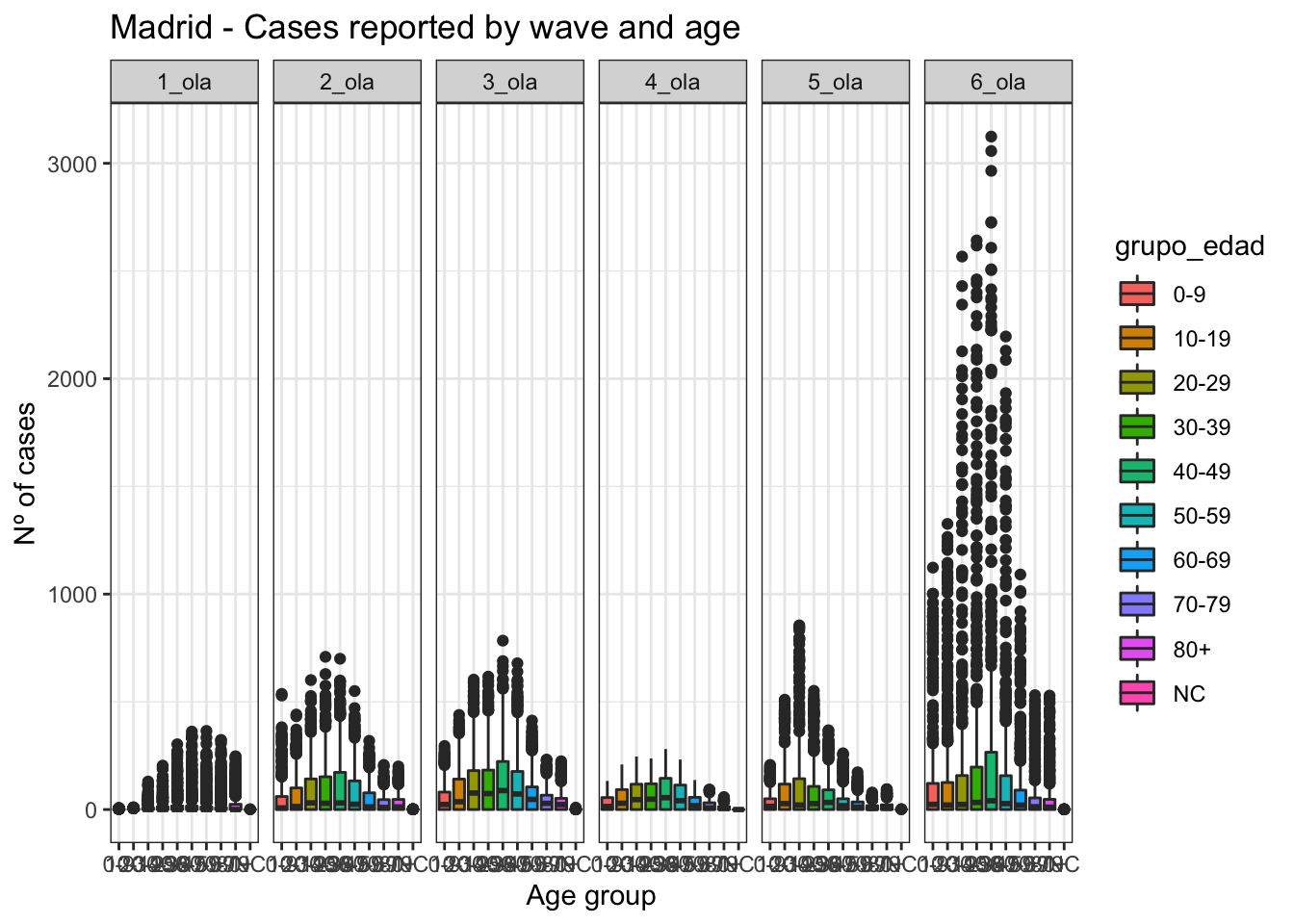
data_Madrid %>%ggplot(aes(x=grupo_edad, y=num_casos)) +geom_boxplot(aes(fill=grupo_edad)) +facet_grid(. ~ ola) +theme(legend.position ="top") +labs(title="Madrid - Cases reported by wave and age",x ="Age group", y ="Nº of cases") +theme_bw()
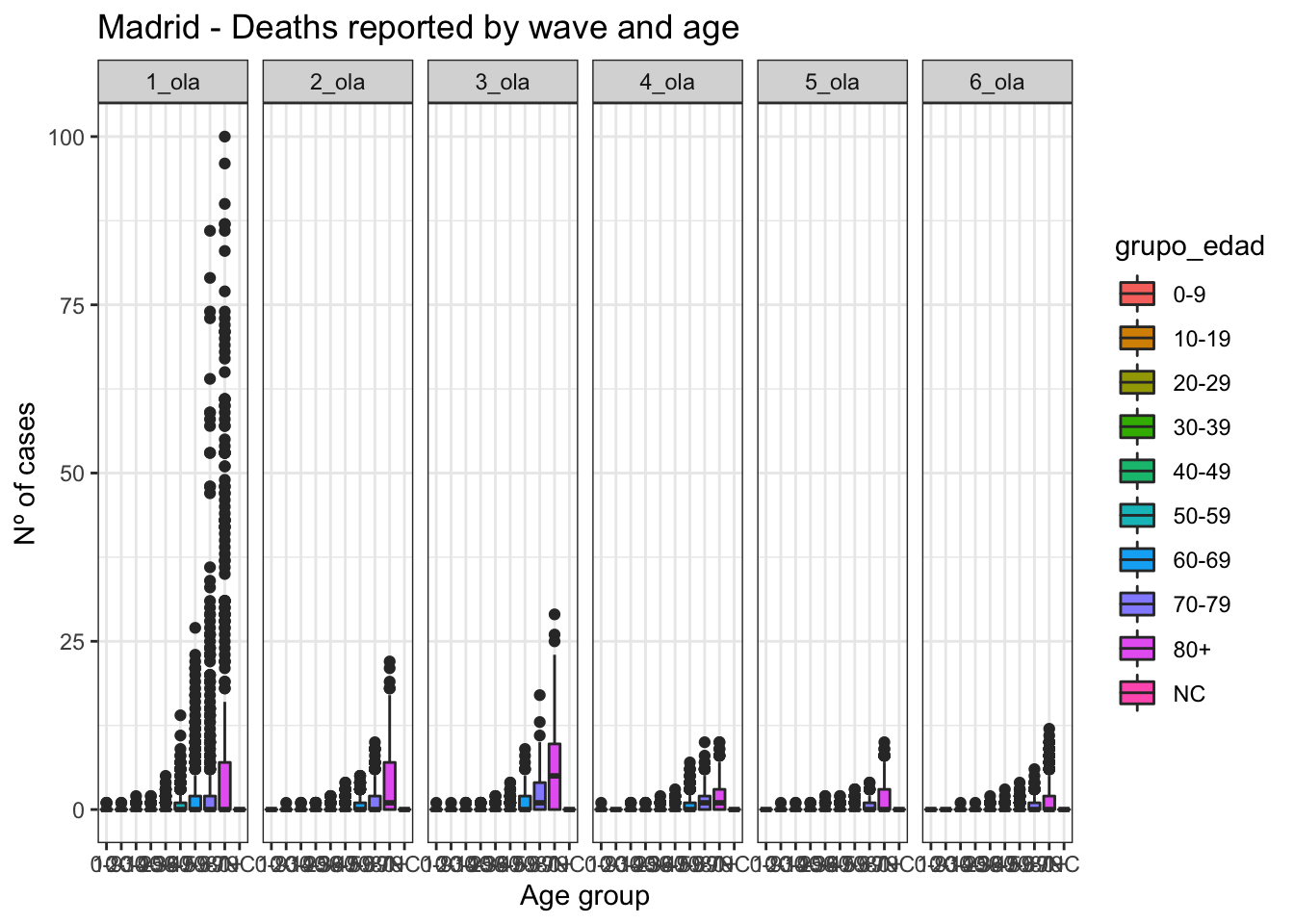
data_Madrid %>%ggplot(aes(x=grupo_edad, y=num_def)) +geom_boxplot(aes(fill=grupo_edad)) +facet_grid(. ~ ola) +theme(legend.position ="top") +labs(title="Madrid - Deaths reported by wave and age",x ="Age group", y ="Nº of cases") +theme_bw()
by age group
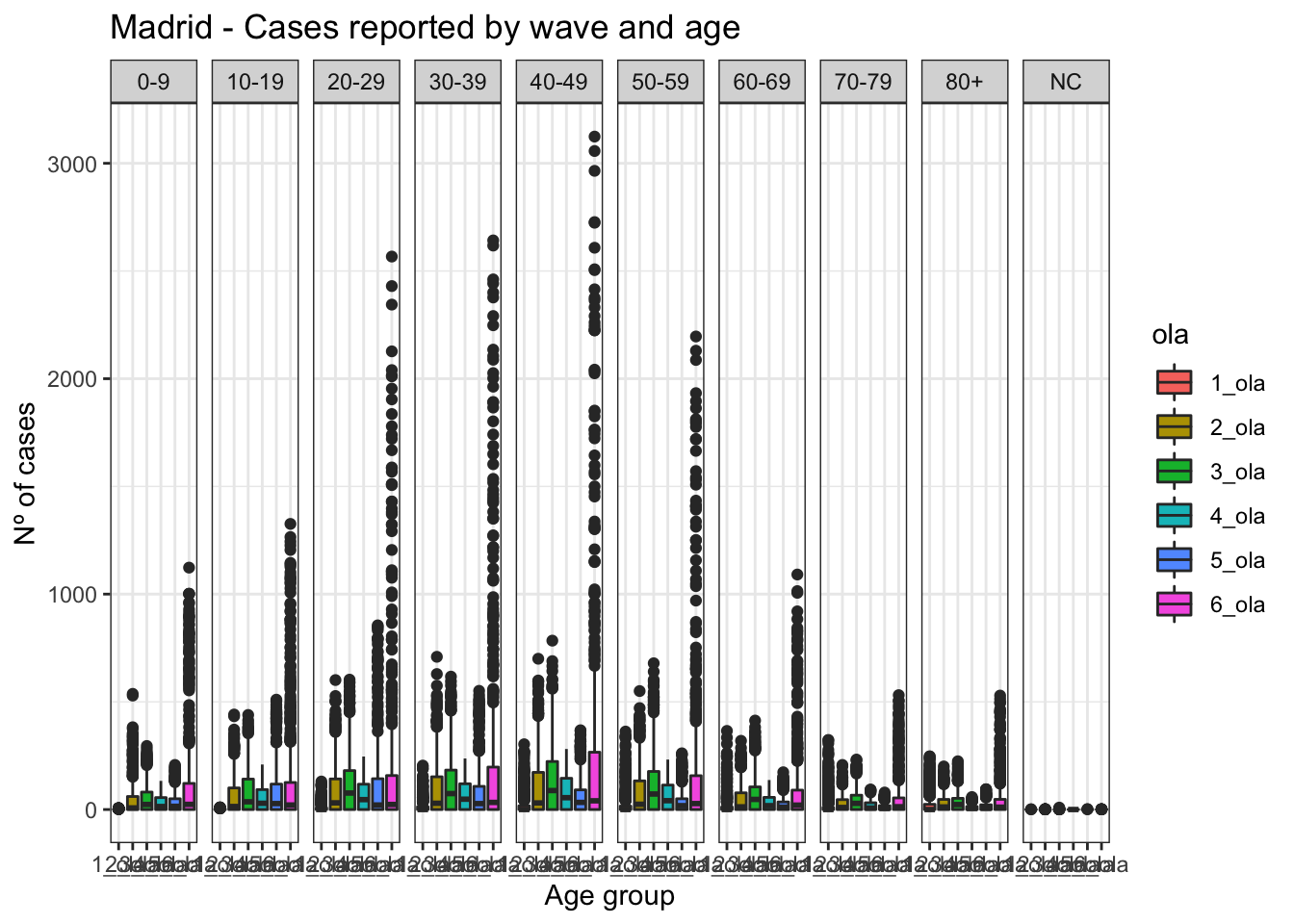
data_Madrid %>%ggplot(aes(x=ola, y=num_casos)) +geom_boxplot(aes(fill=ola)) +facet_grid(. ~ grupo_edad) +theme(legend.position ="top") +labs(title="Madrid - Cases reported by wave and age",x ="Age group", y ="Nº of cases") +theme_bw()
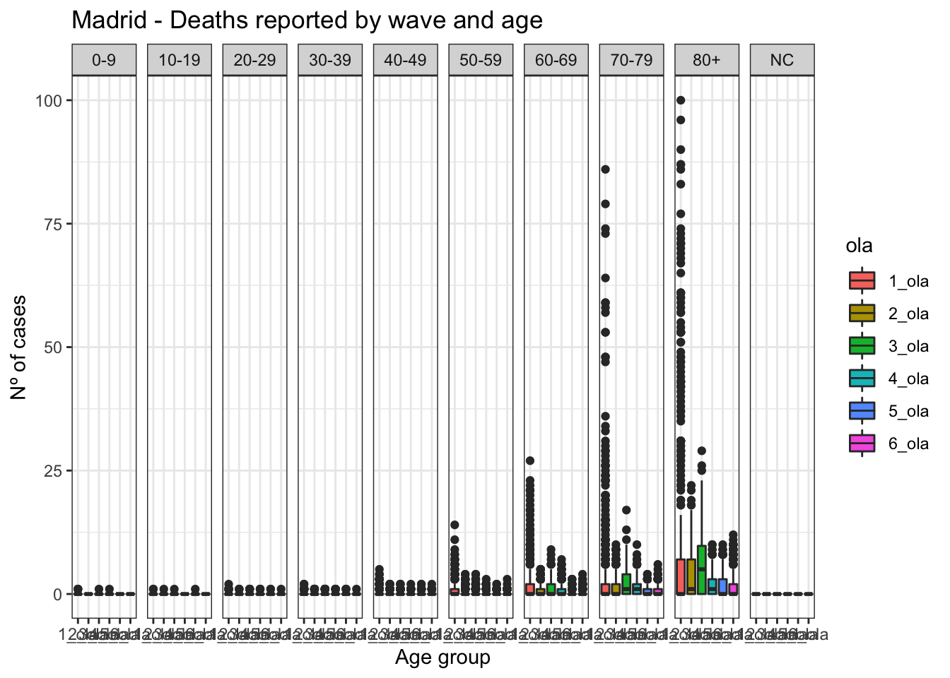
data_Madrid %>%ggplot(aes(x=ola, y=num_def)) +geom_boxplot(aes(fill=ola)) +facet_grid(. ~ grupo_edad) +theme(legend.position ="top") +labs(title="Madrid - Deaths reported by wave and age",x ="Age group", y ="Nº of cases") +theme_bw()
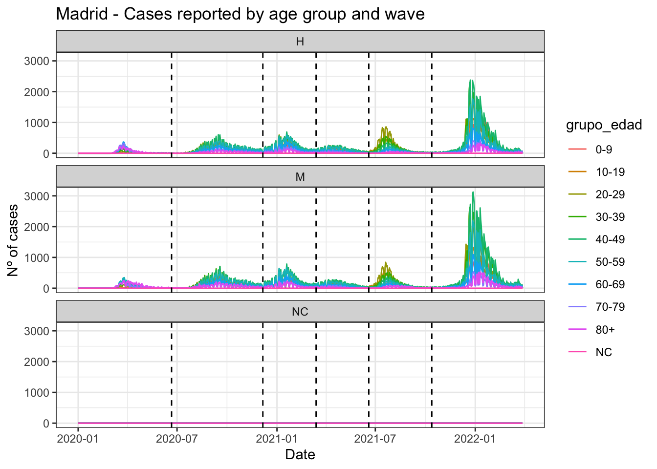
data_Madrid %>%ggplot(aes(x=fecha, y=num_casos)) +geom_line(aes(color=grupo_edad)) +geom_vline(xintercept =as.Date("2020-06-21", format ="%Y-%m-%d"), linetype="dashed") +geom_vline(xintercept =as.Date("2020-12-06", format ="%Y-%m-%d"), linetype="dashed") +geom_vline(xintercept =as.Date("2021-03-14", format ="%Y-%m-%d"), linetype="dashed") +geom_vline(xintercept =as.Date("2021-06-19", format ="%Y-%m-%d"), linetype="dashed") +geom_vline(xintercept =as.Date("2021-10-13", format ="%Y-%m-%d"), linetype="dashed") +facet_wrap(~sexo, ncol=1) +theme(legend.position ="top") +labs(title="Madrid - Cases reported by age group and wave",x ="Date", y ="Nº of cases") +theme_bw()
by sex
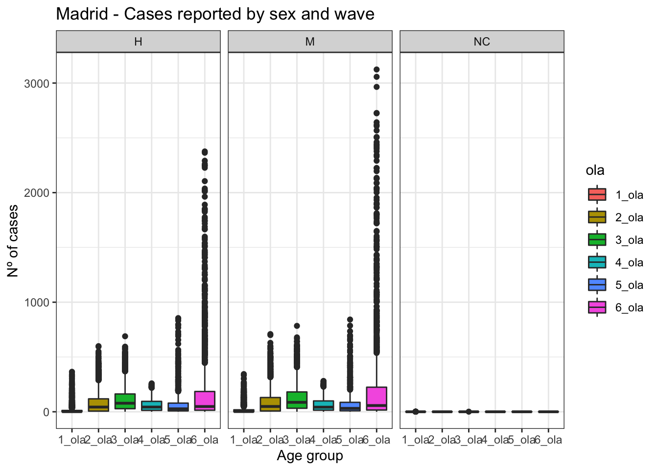
data_Madrid %>%ggplot(aes(x=ola, y=num_casos)) +geom_boxplot(aes(fill=ola)) +facet_grid(. ~ sexo) +theme(legend.position ="top") +labs(title="Madrid - Cases reported by sex and wave",x ="Age group", y ="Nº of cases") +theme_bw()
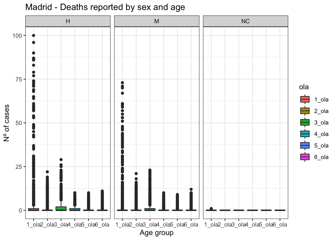
data_Madrid %>%ggplot(aes(x=ola, y=num_def)) +geom_boxplot(aes(fill=ola)) +facet_grid(. ~ sexo) +theme(legend.position ="top") +labs(title="Madrid - Deaths reported by sex and age",x ="Age group", y ="Nº of cases") +theme_bw()
data_Madrid %>%ggplot(aes(x=fecha, y=num_casos)) +geom_line(aes(color=sexo)) +geom_vline(xintercept =as.Date("2020-06-21", format ="%Y-%m-%d"), linetype="dashed") +geom_vline(xintercept =as.Date("2020-12-06", format ="%Y-%m-%d"), linetype="dashed") +geom_vline(xintercept =as.Date("2021-03-14", format ="%Y-%m-%d"), linetype="dashed") +geom_vline(xintercept =as.Date("2021-06-19", format ="%Y-%m-%d"), linetype="dashed") +geom_vline(xintercept =as.Date("2021-10-13", format ="%Y-%m-%d"), linetype="dashed") +facet_wrap(~grupo_edad, scales ="free_y", ncol=1) +theme(legend.position ="top") +labs(title="Madrid - Cases reported by sex and age group (free y axis)",x ="Date", y ="Nº of cases") +theme_bw()
Malaga
data_Malaga <- hosp_data %>%filter(provincia =="Málaga") %>%select(-provincia) %>%as_tsibble(index = fecha, key =c(sexo, grupo_edad)) %>%mutate(ola =case_when( fecha <as.Date("2020-06-21", format ="%Y-%m-%d") ~"1_ola", fecha <as.Date("2020-12-06", format ="%Y-%m-%d") ~"2_ola", fecha <as.Date("2021-03-14", format ="%Y-%m-%d") ~"3_ola", fecha <as.Date("2021-06-19", format ="%Y-%m-%d") ~"4_ola", fecha <as.Date("2021-10-13", format ="%Y-%m-%d") ~"5_ola",TRUE~"6_ola", ))data_Malaga
# A tsibble: 24,570 x 8 [1D]
# Key:       sexo, grupo_edad [30]
   sexo  grupo_edad fecha      num_casos num_hosp num_uci num_def ola
   <chr> <chr>      <date>         <dbl>    <dbl>   <dbl>   <dbl> <chr>
 1 H     0-9        2020-01-01         0        0       0       0 1_ola
 2 H     0-9        2020-01-02         0        0       0       0 1_ola
 3 H     0-9        2020-01-03         0        0       0       0 1_ola
 4 H     0-9        2020-01-04         0        0       0       0 1_ola
 5 H     0-9        2020-01-05         0        0       0       0 1_ola
 6 H     0-9        2020-01-06         0        0       0       0 1_ola
 7 H     0-9        2020-01-07         0        0       0       0 1_ola
 8 H     0-9        2020-01-08         0        0       0       0 1_ola
 9 H     0-9        2020-01-09         0        0       0       0 1_ola
10 H     0-9        2020-01-10         0        0       0       0 1_ola
# … with 24,560 more rows
by wave
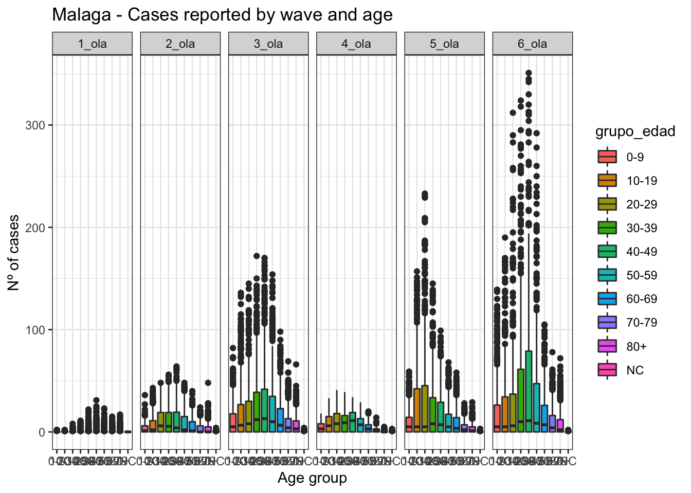
data_Malaga %>%ggplot(aes(x=grupo_edad, y=num_casos)) +geom_boxplot(aes(fill=grupo_edad)) +facet_grid(. ~ ola) +theme(legend.position ="top") +labs(title="Malaga - Cases reported by wave and age",x ="Age group", y ="Nº of cases") +theme_bw()
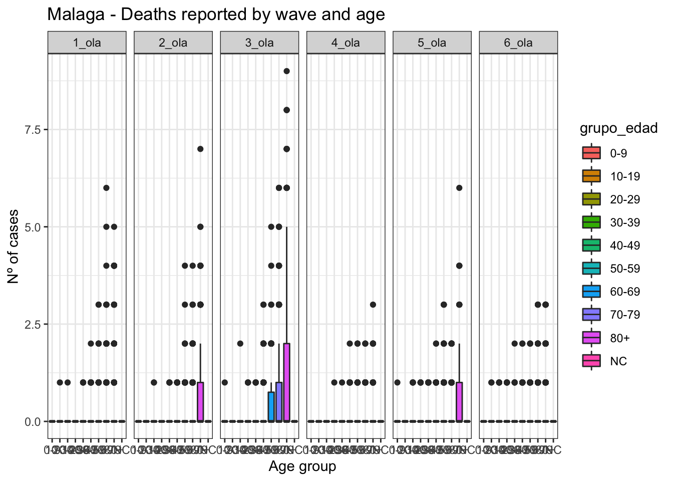
data_Malaga %>%ggplot(aes(x=grupo_edad, y=num_def)) +geom_boxplot(aes(fill=grupo_edad)) +facet_grid(. ~ ola) +theme(legend.position ="top") +labs(title="Malaga - Deaths reported by wave and age",x ="Age group", y ="Nº of cases") +theme_bw()
by age group
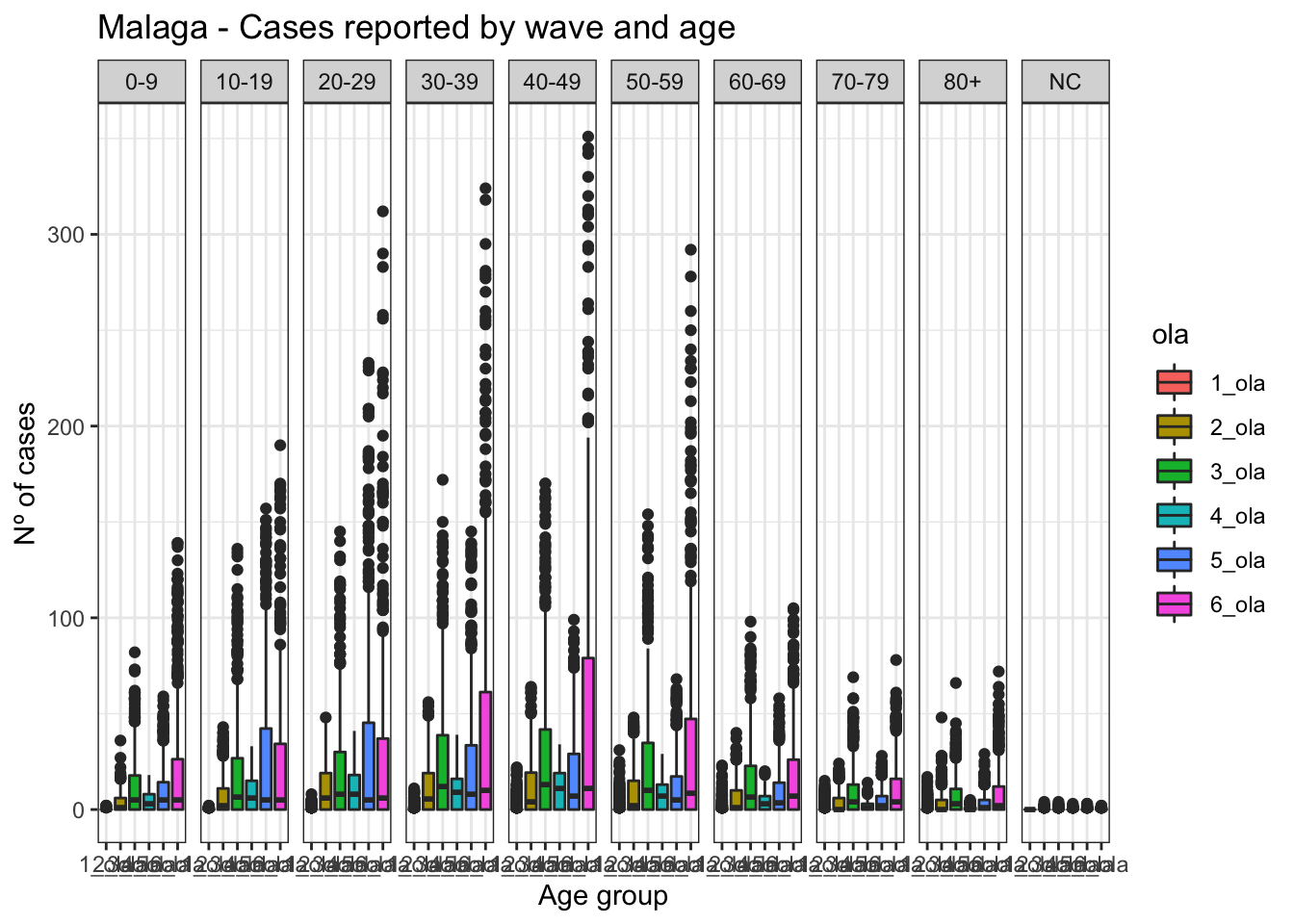
data_Malaga %>%ggplot(aes(x=ola, y=num_casos)) +geom_boxplot(aes(fill=ola)) +facet_grid(. ~ grupo_edad) +theme(legend.position ="top") +labs(title="Malaga - Cases reported by wave and age",x ="Age group", y ="Nº of cases") +theme_bw()
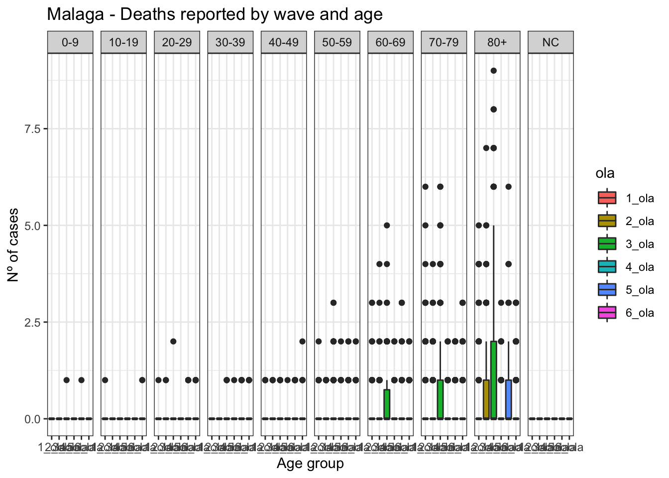
data_Malaga %>%ggplot(aes(x=ola, y=num_def)) +geom_boxplot(aes(fill=ola)) +facet_grid(. ~ grupo_edad) +theme(legend.position ="top") +labs(title="Malaga - Deaths reported by wave and age",x ="Age group", y ="Nº of cases") +theme_bw()
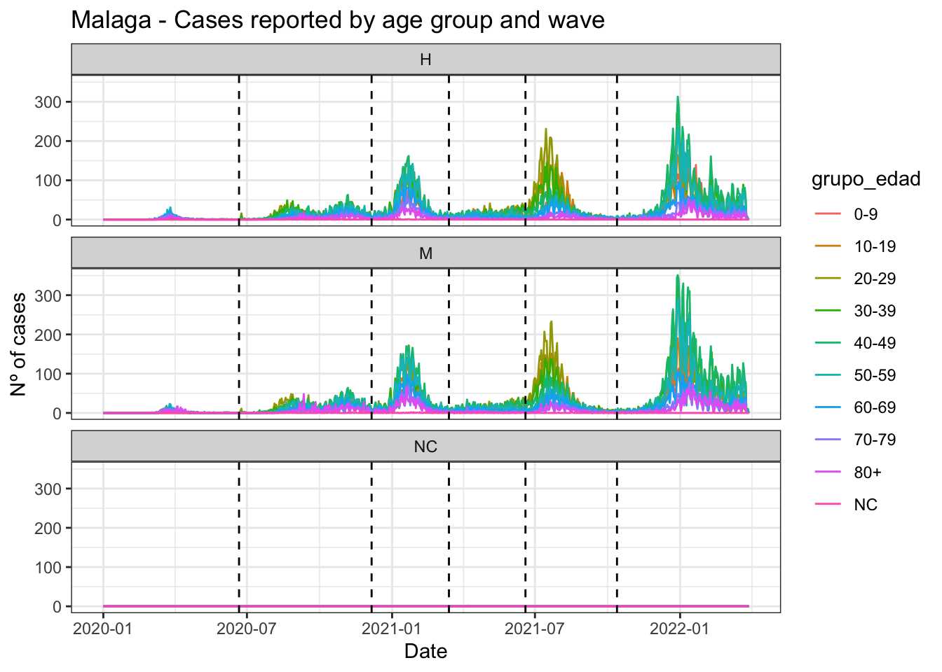
data_Malaga %>%ggplot(aes(x=fecha, y=num_casos)) +geom_line(aes(color=grupo_edad)) +geom_vline(xintercept =as.Date("2020-06-21", format ="%Y-%m-%d"), linetype="dashed") +geom_vline(xintercept =as.Date("2020-12-06", format ="%Y-%m-%d"), linetype="dashed") +geom_vline(xintercept =as.Date("2021-03-14", format ="%Y-%m-%d"), linetype="dashed") +geom_vline(xintercept =as.Date("2021-06-19", format ="%Y-%m-%d"), linetype="dashed") +geom_vline(xintercept =as.Date("2021-10-13", format ="%Y-%m-%d"), linetype="dashed") +facet_wrap(~sexo, ncol=1) +theme(legend.position ="top") +labs(title="Malaga - Cases reported by age group and wave",x ="Date", y ="Nº of cases") +theme_bw()
by sex
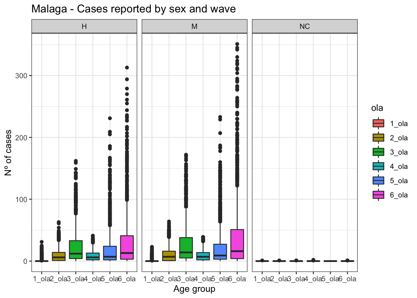
data_Malaga %>%ggplot(aes(x=ola, y=num_casos)) +geom_boxplot(aes(fill=ola)) +facet_grid(. ~ sexo) +theme(legend.position ="top") +labs(title="Malaga - Cases reported by sex and wave",x ="Age group", y ="Nº of cases") +theme_bw()
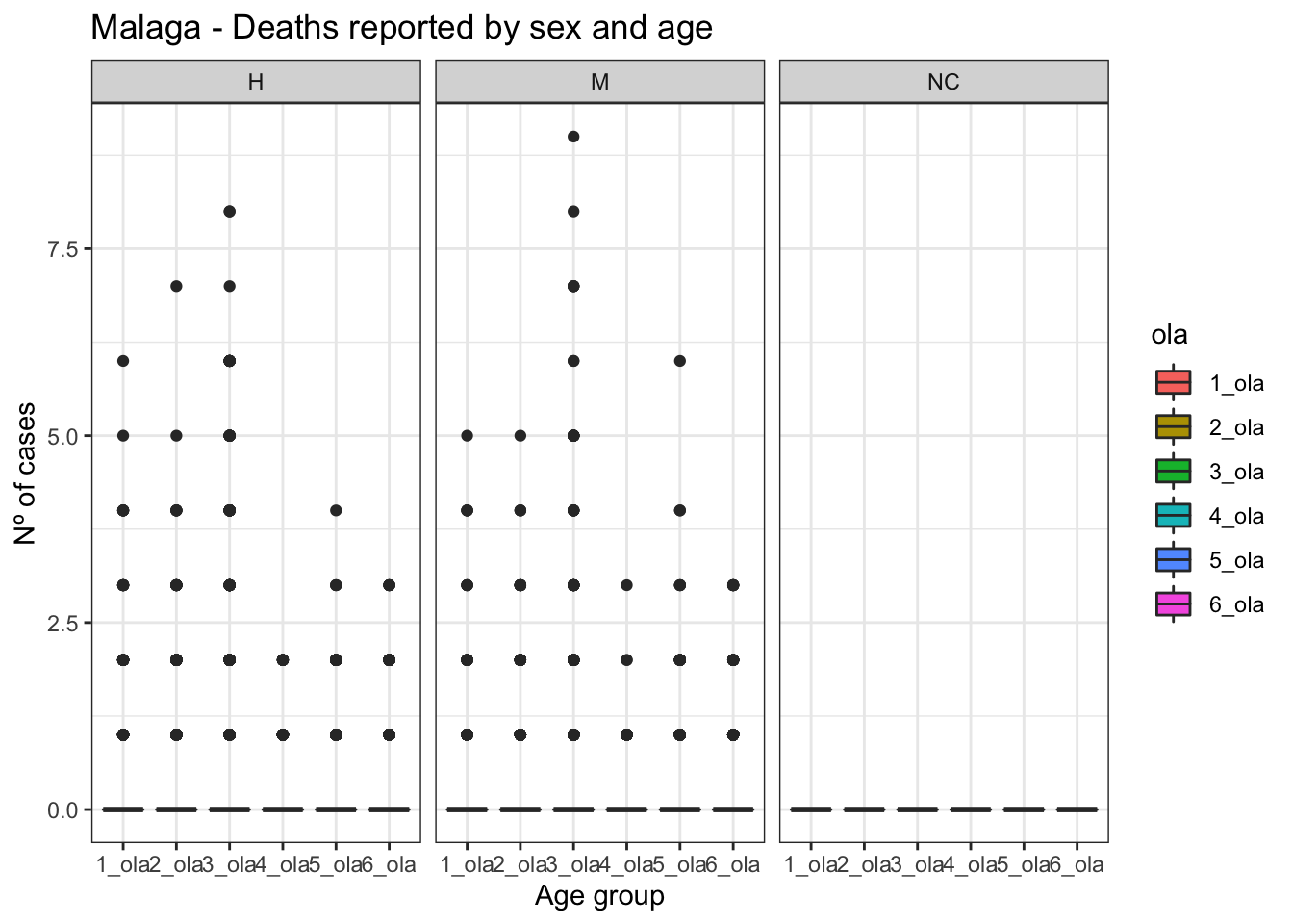
data_Malaga %>%ggplot(aes(x=ola, y=num_def)) +geom_boxplot(aes(fill=ola)) +facet_grid(. ~ sexo) +theme(legend.position ="top") +labs(title="Malaga - Deaths reported by sex and age",x ="Age group", y ="Nº of cases") +theme_bw()
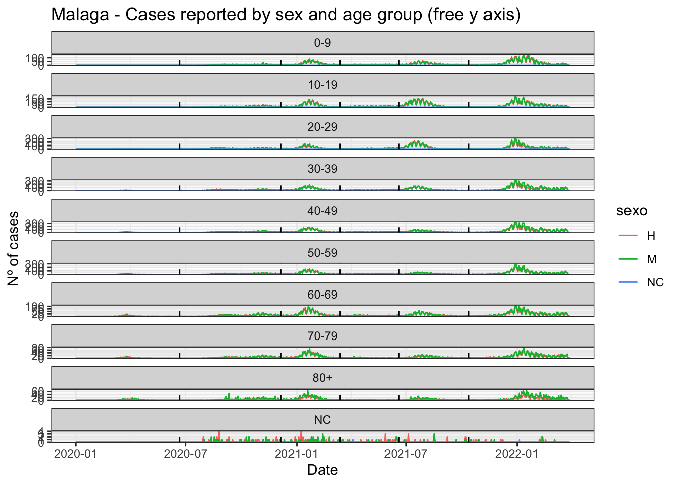
data_Malaga %>%ggplot(aes(x=fecha, y=num_casos)) +geom_line(aes(color=sexo)) +geom_vline(xintercept =as.Date("2020-06-21", format ="%Y-%m-%d"), linetype="dashed") +geom_vline(xintercept =as.Date("2020-12-06", format ="%Y-%m-%d"), linetype="dashed") +geom_vline(xintercept =as.Date("2021-03-14", format ="%Y-%m-%d"), linetype="dashed") +geom_vline(xintercept =as.Date("2021-06-19", format ="%Y-%m-%d"), linetype="dashed") +geom_vline(xintercept =as.Date("2021-10-13", format ="%Y-%m-%d"), linetype="dashed") +facet_wrap(~grupo_edad, scales ="free_y", ncol=1) +theme(legend.position ="top") +labs(title="Malaga - Cases reported by sex and age group (free y axis)",x ="Date", y ="Nº of cases") +theme_bw()
Sevilla
data_Sevilla <- hosp_data %>%filter(provincia =="Sevilla") %>%select(-provincia) %>%as_tsibble(index = fecha, key =c(sexo, grupo_edad)) %>%mutate(ola =case_when( fecha <as.Date("2020-06-21", format ="%Y-%m-%d") ~"1_ola", fecha <as.Date("2020-12-06", format ="%Y-%m-%d") ~"2_ola", fecha <as.Date("2021-03-14", format ="%Y-%m-%d") ~"3_ola", fecha <as.Date("2021-06-19", format ="%Y-%m-%d") ~"4_ola", fecha <as.Date("2021-10-13", format ="%Y-%m-%d") ~"5_ola",TRUE~"6_ola", ))data_Sevilla
# A tsibble: 24,570 x 8 [1D]
# Key:       sexo, grupo_edad [30]
   sexo  grupo_edad fecha      num_casos num_hosp num_uci num_def ola
   <chr> <chr>      <date>         <dbl>    <dbl>   <dbl>   <dbl> <chr>
 1 H     0-9        2020-01-01         0        0       0       0 1_ola
 2 H     0-9        2020-01-02         0        0       0       0 1_ola
 3 H     0-9        2020-01-03         0        0       0       0 1_ola
 4 H     0-9        2020-01-04         0        0       0       0 1_ola
 5 H     0-9        2020-01-05         0        0       0       0 1_ola
 6 H     0-9        2020-01-06         0        0       0       0 1_ola
 7 H     0-9        2020-01-07         0        0       0       0 1_ola
 8 H     0-9        2020-01-08         0        0       0       0 1_ola
 9 H     0-9        2020-01-09         0        0       0       0 1_ola
10 H     0-9        2020-01-10         0        0       0       0 1_ola
# … with 24,560 more rows
by wave
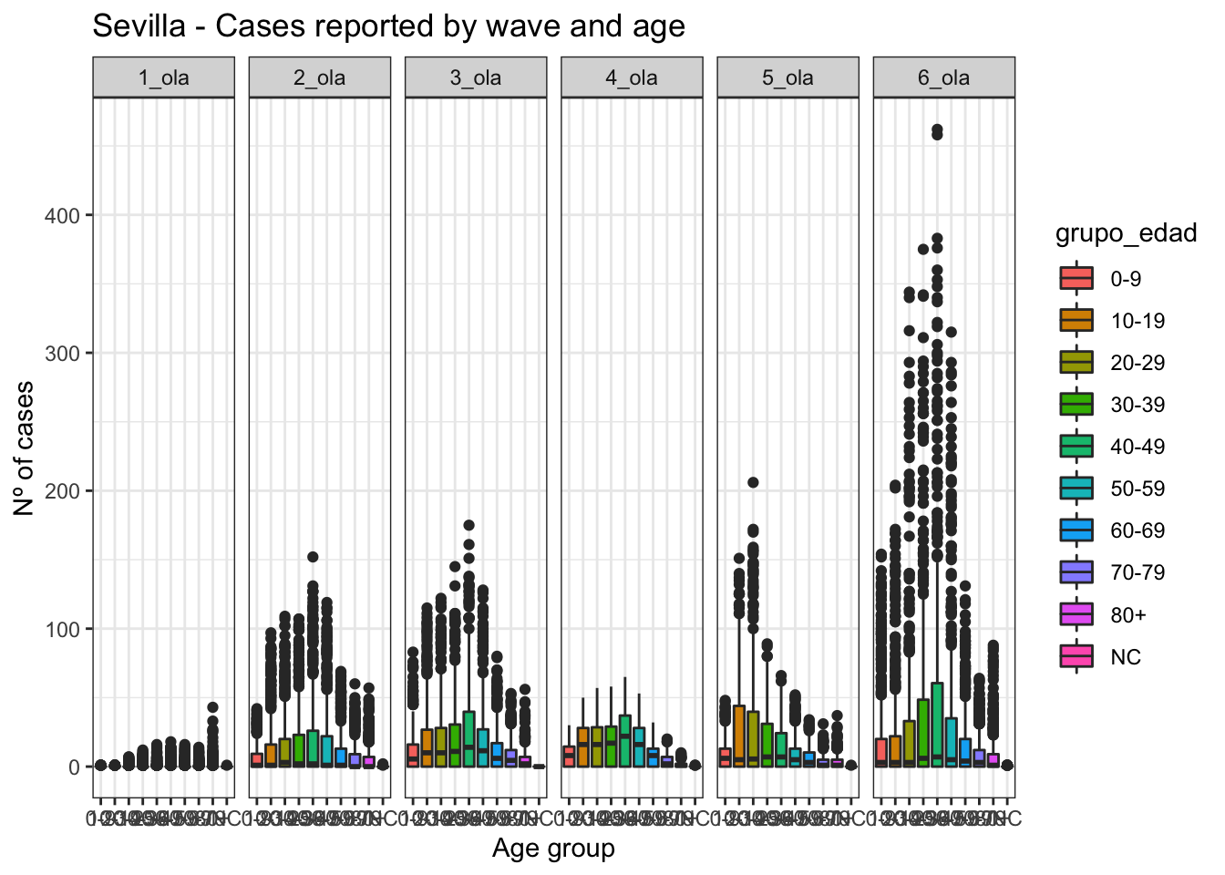
data_Sevilla %>%ggplot(aes(x=grupo_edad, y=num_casos)) +geom_boxplot(aes(fill=grupo_edad)) +facet_grid(. ~ ola) +theme(legend.position ="top") +labs(title="Sevilla - Cases reported by wave and age",x ="Age group", y ="Nº of cases") +theme_bw()
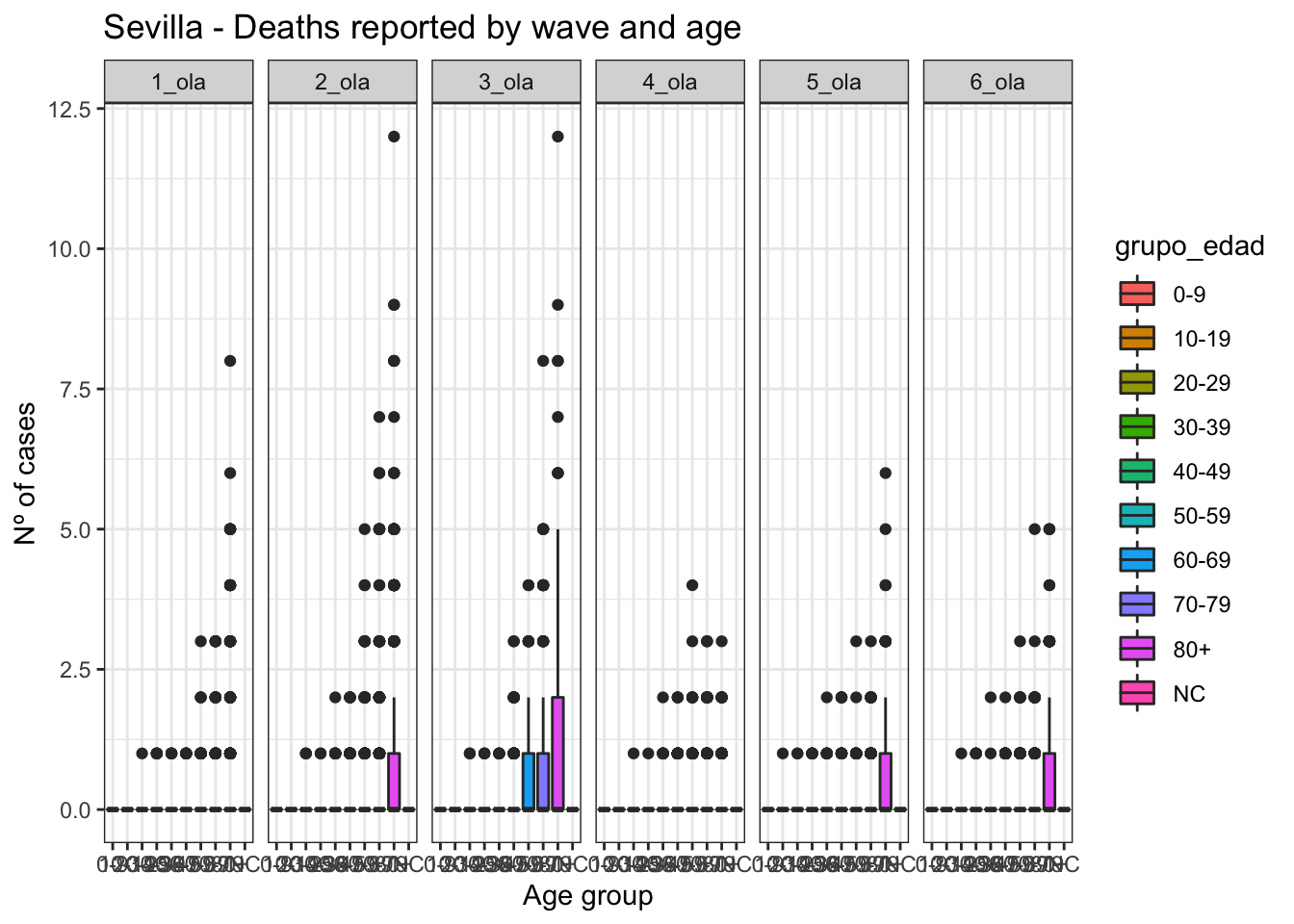
data_Sevilla %>%ggplot(aes(x=grupo_edad, y=num_def)) +geom_boxplot(aes(fill=grupo_edad)) +facet_grid(. ~ ola) +theme(legend.position ="top") +labs(title="Sevilla - Deaths reported by wave and age",x ="Age group", y ="Nº of cases") +theme_bw()
by age group
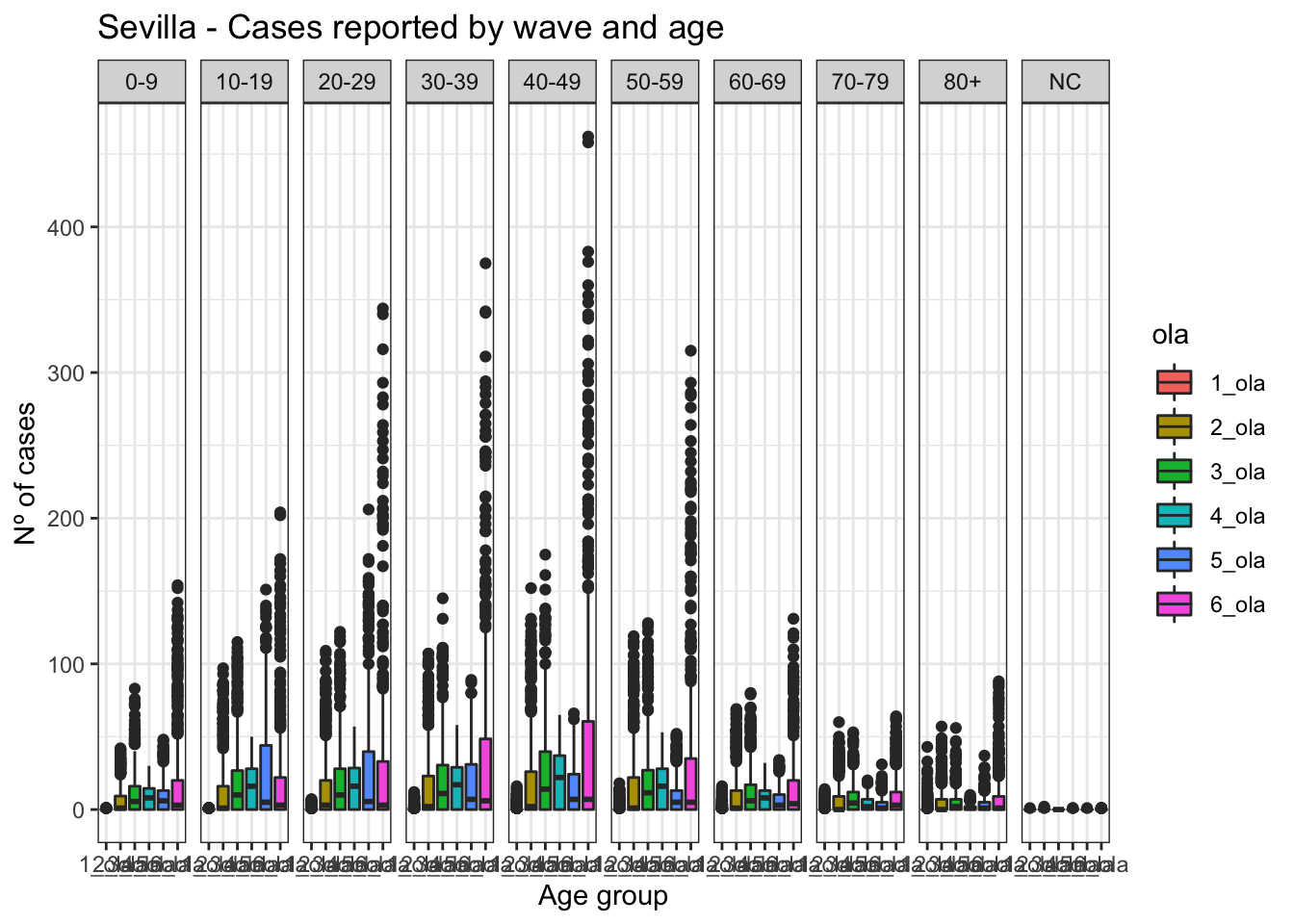
data_Sevilla %>%ggplot(aes(x=ola, y=num_casos)) +geom_boxplot(aes(fill=ola)) +facet_grid(. ~ grupo_edad) +theme(legend.position ="top") +labs(title="Sevilla - Cases reported by wave and age",x ="Age group", y ="Nº of cases") +theme_bw()
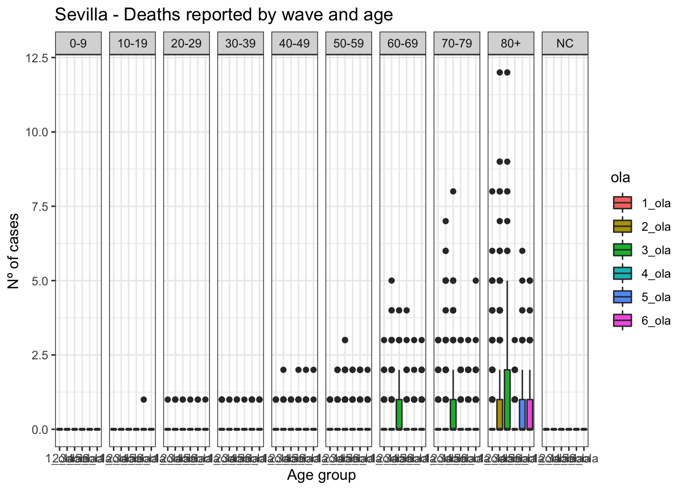
data_Sevilla %>%ggplot(aes(x=ola, y=num_def)) +geom_boxplot(aes(fill=ola)) +facet_grid(. ~ grupo_edad) +theme(legend.position ="top") +labs(title="Sevilla - Deaths reported by wave and age",x ="Age group", y ="Nº of cases") +theme_bw()
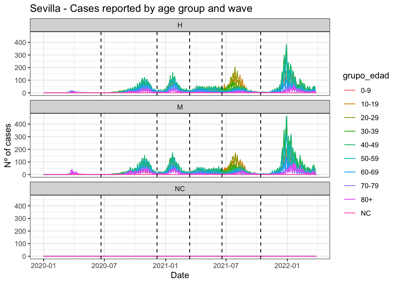
data_Sevilla %>%ggplot(aes(x=fecha, y=num_casos)) +geom_line(aes(color=grupo_edad)) +geom_vline(xintercept =as.Date("2020-06-21", format ="%Y-%m-%d"), linetype="dashed") +geom_vline(xintercept =as.Date("2020-12-06", format ="%Y-%m-%d"), linetype="dashed") +geom_vline(xintercept =as.Date("2021-03-14", format ="%Y-%m-%d"), linetype="dashed") +geom_vline(xintercept =as.Date("2021-06-19", format ="%Y-%m-%d"), linetype="dashed") +geom_vline(xintercept =as.Date("2021-10-13", format ="%Y-%m-%d"), linetype="dashed") +facet_wrap(~sexo, ncol=1) +theme(legend.position ="top") +labs(title="Sevilla - Cases reported by age group and wave",x ="Date", y ="Nº of cases") +theme_bw()
by sex
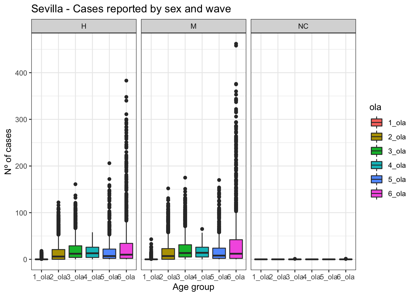
data_Sevilla %>%ggplot(aes(x=ola, y=num_casos)) +geom_boxplot(aes(fill=ola)) +facet_grid(. ~ sexo) +theme(legend.position ="top") +labs(title="Sevilla - Cases reported by sex and wave",x ="Age group", y ="Nº of cases") +theme_bw()
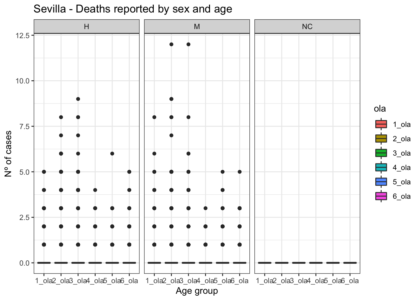
data_Sevilla %>%ggplot(aes(x=ola, y=num_def)) +geom_boxplot(aes(fill=ola)) +facet_grid(. ~ sexo) +theme(legend.position ="top") +labs(title="Sevilla - Deaths reported by sex and age",x ="Age group", y ="Nº of cases") +theme_bw()
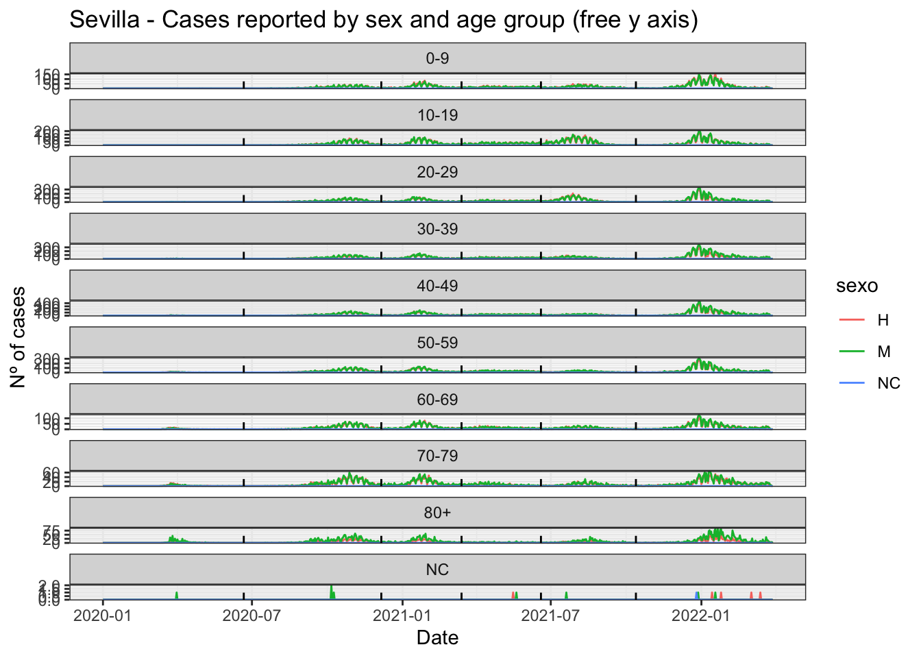
data_Sevilla %>%ggplot(aes(x=fecha, y=num_casos)) +geom_line(aes(color=sexo)) +geom_vline(xintercept =as.Date("2020-06-21", format ="%Y-%m-%d"), linetype="dashed") +geom_vline(xintercept =as.Date("2020-12-06", format ="%Y-%m-%d"), linetype="dashed") +geom_vline(xintercept =as.Date("2021-03-14", format ="%Y-%m-%d"), linetype="dashed") +geom_vline(xintercept =as.Date("2021-06-19", format ="%Y-%m-%d"), linetype="dashed") +geom_vline(xintercept =as.Date("2021-10-13", format ="%Y-%m-%d"), linetype="dashed") +facet_wrap(~grupo_edad, scales ="free_y", ncol=1) +theme(legend.position ="top") +labs(title="Sevilla - Cases reported by sex and age group (free y axis)",x ="Date", y ="Nº of cases") +theme_bw()