pacman::p_load(
      here,      # file locator
      tidyverse, # data management and ggplot2 graphics
      skimr,     # get overview of data
      janitor,   # produce and adorn tabulations and cross-tabulations
      tsibble,
      fable,
      feasts,
      fabletools,
      lubridate
)

covid_data <- readRDS(here("data", "clean", "final_covid_data.rds"))Multivariate (INE mobility + temp) prediction
Load packages:
The temporal limits of our prediction will be:
- Data as of June 14th 2020 which is considered the beginning of the second epidemiological period in Spain
- In the first case scenario, data previous the start of the sixth wave of covid-19 (14 oct 2021).
- In the second case scenario, all the available data (limited by mobility information 29 dec 2021)
Before sixth epidemiological period
Asturias
data_asturias <- covid_data %>%
      filter(provincia == "Asturias") %>%
      filter(fecha > as.Date("2020-06-14", format = "%Y-%m-%d")) %>%
      select(provincia, fecha, num_casos, tmed, mob_flujo) %>%
      drop_na() %>%
      as_tsibble(key = provincia, index = fecha)
data_asturias
# A tsibble: 563 x 5 [1D]
# Key: provincia [1]
provincia fecha num_casos tmed mob_flujo
<chr> <date> <dbl> <dbl> <dbl>
1 Asturias 2020-06-15 0 16 19.4
2 Asturias 2020-06-16 1 15.6 19.5
3 Asturias 2020-06-17 0 15.6 19.7
4 Asturias 2020-06-18 0 15.1 20.5
5 Asturias 2020-06-19 0 14.8 21.0
6 Asturias 2020-06-20 0 16.8 19.8
7 Asturias 2020-06-21 0 18.2 20.2
8 Asturias 2020-06-22 0 18.2 20.6
9 Asturias 2020-06-23 0 20 21.1
10 Asturias 2020-06-24 0 18.2 21.5
# … with 553 more rowsdata_asturias_train <- data_asturias %>%
filter(fecha <= as.Date("2021-10-14", format = "%Y-%m-%d"))
summary(data_asturias_train$fecha) Min. 1st Qu. Median Mean 3rd Qu. Max.
"2020-06-15" "2020-10-14" "2021-02-13" "2021-02-13" "2021-06-14" "2021-10-14" data_asturias_test <- data_asturias %>%
filter(fecha > as.Date("2021-10-14", format = "%Y-%m-%d"))
summary(data_asturias_test$fecha) Min. 1st Qu. Median Mean 3rd Qu. Max.
"2021-10-15" "2021-11-02" "2021-11-21" "2021-11-21" "2021-12-10" "2021-12-29" # Lamba for num_casos
lambda_asturias_casos <- data_asturias %>%
features(num_casos, features = guerrero) %>%
pull(lambda_guerrero)
lambda_asturias_casos[1] 0.2493395# Lamba for average temp
lambda_asturias_tmed <- data_asturias %>%
features(tmed, features = guerrero) %>%
pull(lambda_guerrero)
lambda_asturias_tmed[1] 1.142823# Lamba for mobility
lambda_asturias_mobil <- data_asturias %>%
features(mob_flujo, features = guerrero) %>%
pull(lambda_guerrero)
lambda_asturias_mobil[1] 1.459993fit_model <- data_asturias_train %>%
model(
arima_at1 = ARIMA(box_cox(num_casos, lambda_asturias_casos) ~
box_cox(tmed, lambda_asturias_tmed) +
box_cox(mob_flujo, lambda_asturias_mobil)),
arima_at2 = ARIMA(box_cox(num_casos, lambda_asturias_casos) ~
box_cox(tmed, lambda_asturias_tmed) +
box_cox(mob_flujo, lambda_asturias_mobil),
stepwise = FALSE, approx = FALSE),
Snaive = SNAIVE(box_cox(num_casos, lambda_asturias_casos))
)
# Show and report model
fit_model# A mable: 1 x 4
# Key: provincia [1]
provincia arima_at1
<chr> <model>
1 Asturias <LM w/ ARIMA(2,0,2)(0,1,1)[7] errors>
# … with 2 more variables: arima_at2 <model>, Snaive <model>glance(fit_model)# A tibble: 3 × 9
provincia .model sigma2 log_lik AIC AICc BIC ar_roots ma_roots
<chr> <chr> <dbl> <dbl> <dbl> <dbl> <dbl> <list> <list>
1 Asturias arima_at1 1.02 -687. 1392. 1392. 1429. <cpl [2]> <cpl [9]>
2 Asturias arima_at2 1.00 -683. 1386. 1386. 1428. <cpl [9]> <cpl [15]>
3 Asturias Snaive 2.66 NA NA NA NA <NULL> <NULL> fit_model %>%
pivot_longer(-provincia,
names_to = ".model",
values_to = "orders") %>%
left_join(glance(fit_model), by = c("provincia", ".model")) %>%
arrange(AICc) %>%
select(.model:BIC)# A mable: 3 x 7
# Key: .model [3]
.model orders sigma2 log_lik AIC AICc BIC
<chr> <model> <dbl> <dbl> <dbl> <dbl> <dbl>
1 arima_… <LM w/ ARIMA(2,0,1)(1,1,2)[7] errors> 1.00 -683. 1386. 1386. 1428.
2 arima_… <LM w/ ARIMA(2,0,2)(0,1,1)[7] errors> 1.02 -687. 1392. 1392. 1429.
3 Snaive <SNAIVE> 2.66 NA NA NA NA # We use a Ljung-Box test >> large p-value, confirms residuals are similar / considered to white noise
fit_model %>%
select(Snaive) %>%
gg_tsresiduals()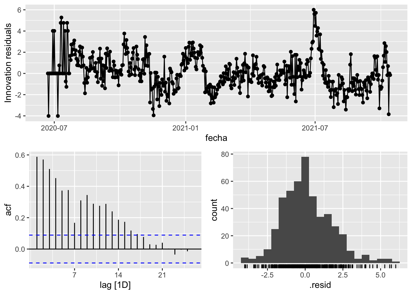
fit_model %>%
      select(arima_at1) %>%
      gg_tsresiduals()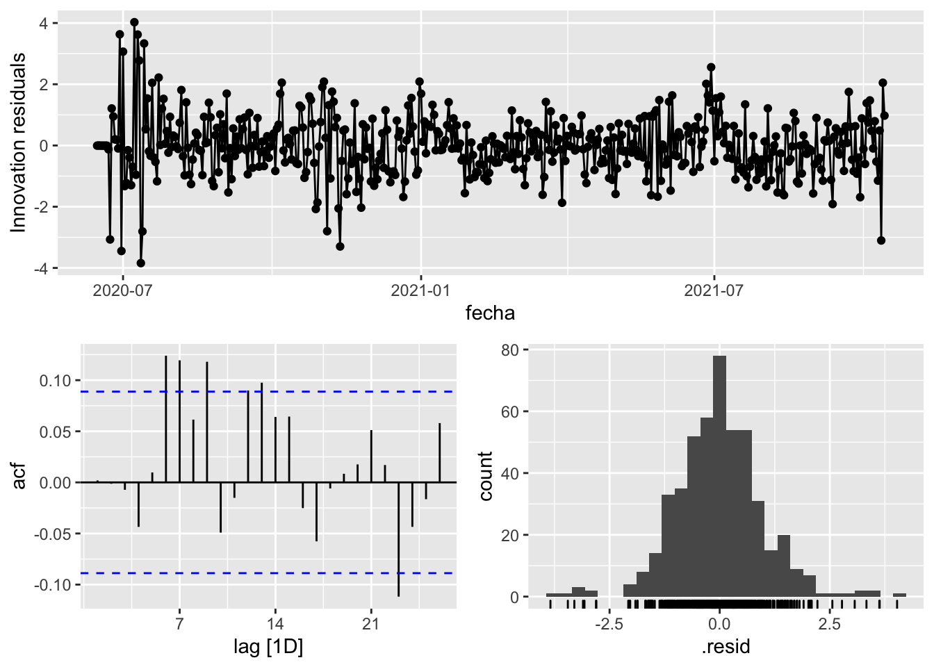
fit_model %>%
      select(arima_at2) %>%
      gg_tsresiduals()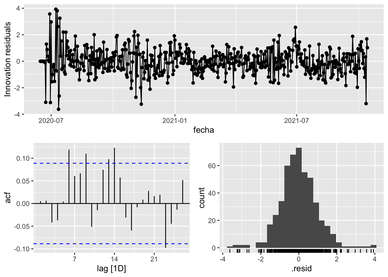
augment(fit_model) %>%
      features(.innov, ljung_box, lag=7)
# A tibble: 3 × 4
provincia .model lb_stat lb_pvalue
<chr> <chr> <dbl> <dbl>
1 Asturias arima_at1 15.7 0.0281
2 Asturias arima_at2 10.4 0.166
3 Asturias Snaive 701. 0 augment(fit_model) %>%
features(.innov, ljung_box, lag=14)# A tibble: 3 × 4
provincia .model lb_stat lb_pvalue
<chr> <chr> <dbl> <dbl>
1 Asturias arima_at1 36.7 0.000812
2 Asturias arima_at2 35.3 0.00132
3 Asturias Snaive 972. 0 augment(fit_model) %>%
features(.innov, ljung_box, lag=21)# A tibble: 3 × 4
provincia .model lb_stat lb_pvalue
<chr> <chr> <dbl> <dbl>
1 Asturias arima_at1 42.4 0.00377
2 Asturias arima_at2 39.9 0.00773
3 Asturias Snaive 1003. 0 augment(fit_model) %>%
features(.innov, ljung_box, lag=90)# A tibble: 3 × 4
provincia .model lb_stat lb_pvalue
<chr> <chr> <dbl> <dbl>
1 Asturias arima_at1 110. 0.0782
2 Asturias arima_at2 96.9 0.290
3 Asturias Snaive 1324. 0 # To predict future values of infections, we need to pass the model future/prediction values of the complementary variables tmed and mobility
# We are going to select those from the test dataset
data_fc_h7 <- data_asturias_test %>%
select(-num_casos) %>%
slice(1:7)
data_fc_h14 <- data_asturias_test %>%
select(-num_casos) %>%
slice(1:14)
data_fc_h21 <- data_asturias_test %>%
select(-num_casos) %>%
slice(1:21)
data_fc_h90 <- data_asturias_test %>%
select(-num_casos) %>%
slice(1:90)# Significant spikes out of 30 is still consistent with white noise
# To be sure, use a Ljung-Box test, which has a large p-value, confirming that
# the residuals are similar to white noise.
# Note that the alternative models also passed this test.
#
# Forecast
fc_h7 <- fabletools::forecast(fit_model, new_data = data_fc_h7)
fc_h14 <- fabletools::forecast(fit_model, new_data = data_fc_h14)
fc_h21 <- fabletools::forecast(fit_model, new_data = data_fc_h21)
fc_h90 <- fabletools::forecast(fit_model, new_data = data_fc_h90)7 days
# Plots
fc_h7 %>%
      autoplot(
            data_asturias_test %>%
                  filter(fecha <= as.Date("2021-10-14", format = "%Y-%m-%d")+days(7))
      ) +
      labs(y = "Nº cases", title = "Asturias - forecast h7")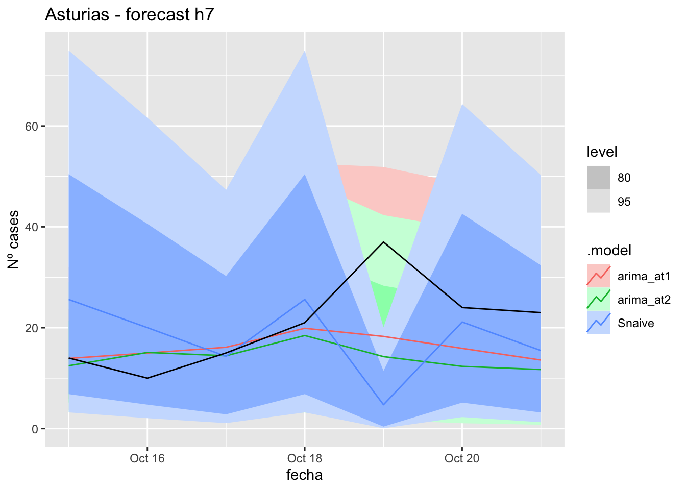
fc_h7 %>%
      autoplot(
            data_asturias %>%
                  filter(fecha <= as.Date("2021-10-14", format = "%Y-%m-%d")+days(7) &
                               fecha > as.Date("2021-07-01", format = "%Y-%m-%d"))
      ) +
      labs(y = "Nº cases", title = "Asturias - forecast h7")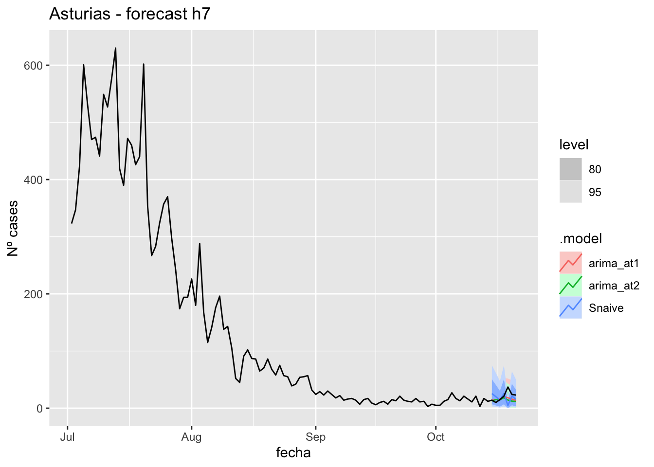
# Accuracy
fabletools::accuracy(fc_h7, data_asturias)
# A tibble: 3 × 11
.model provincia .type ME RMSE MAE MPE MAPE MASE RMSSE ACF1
<chr> <chr> <chr> <dbl> <dbl> <dbl> <dbl> <dbl> <dbl> <dbl> <dbl>
1 arima_at1 Asturias Test 4.47 8.72 6.22 10.5 26.9 0.125 0.106 0.344
2 arima_at2 Asturias Test 6.46 10.8 7.91 19.3 33.8 0.159 0.131 0.371
3 Snaive Asturias Test 2.44 14.0 9.93 -9.80 48.8 0.200 0.170 0.010614 days
# Plots
fc_h14 %>%
      autoplot(
            data_asturias_test %>%
                  filter(fecha <= as.Date("2021-10-14", format = "%Y-%m-%d")+days(14))
      ) +
      labs(y = "Nº cases", title = "Asturias - forecast h14")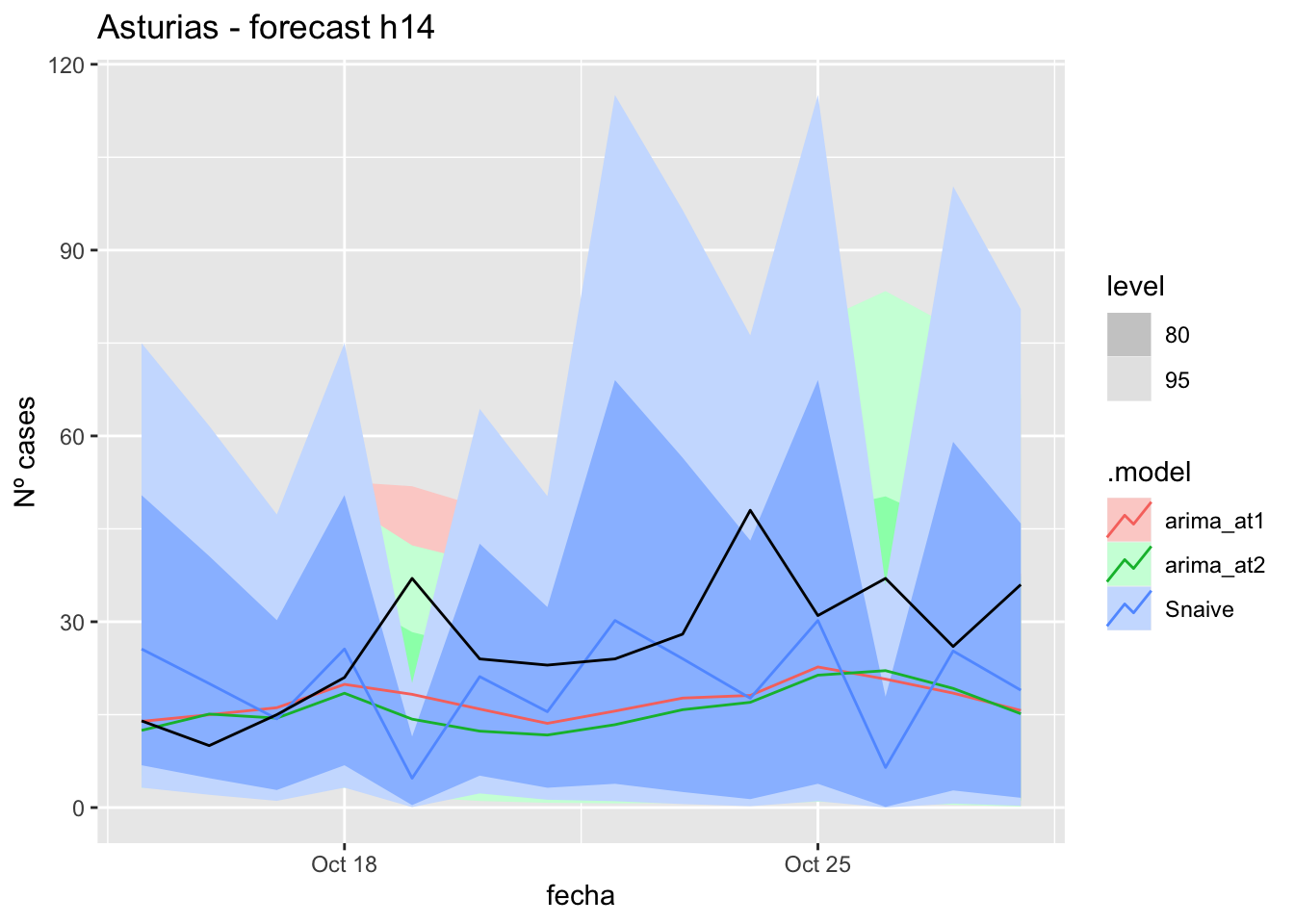
fc_h14 %>%
      autoplot(
            data_asturias %>%
                  filter(fecha <= as.Date("2021-10-14", format = "%Y-%m-%d")+days(14) &
                               fecha > as.Date("2021-07-01", format = "%Y-%m-%d"))
      ) +
      labs(y = "Nº cases", title = "Asturias - forecast h14")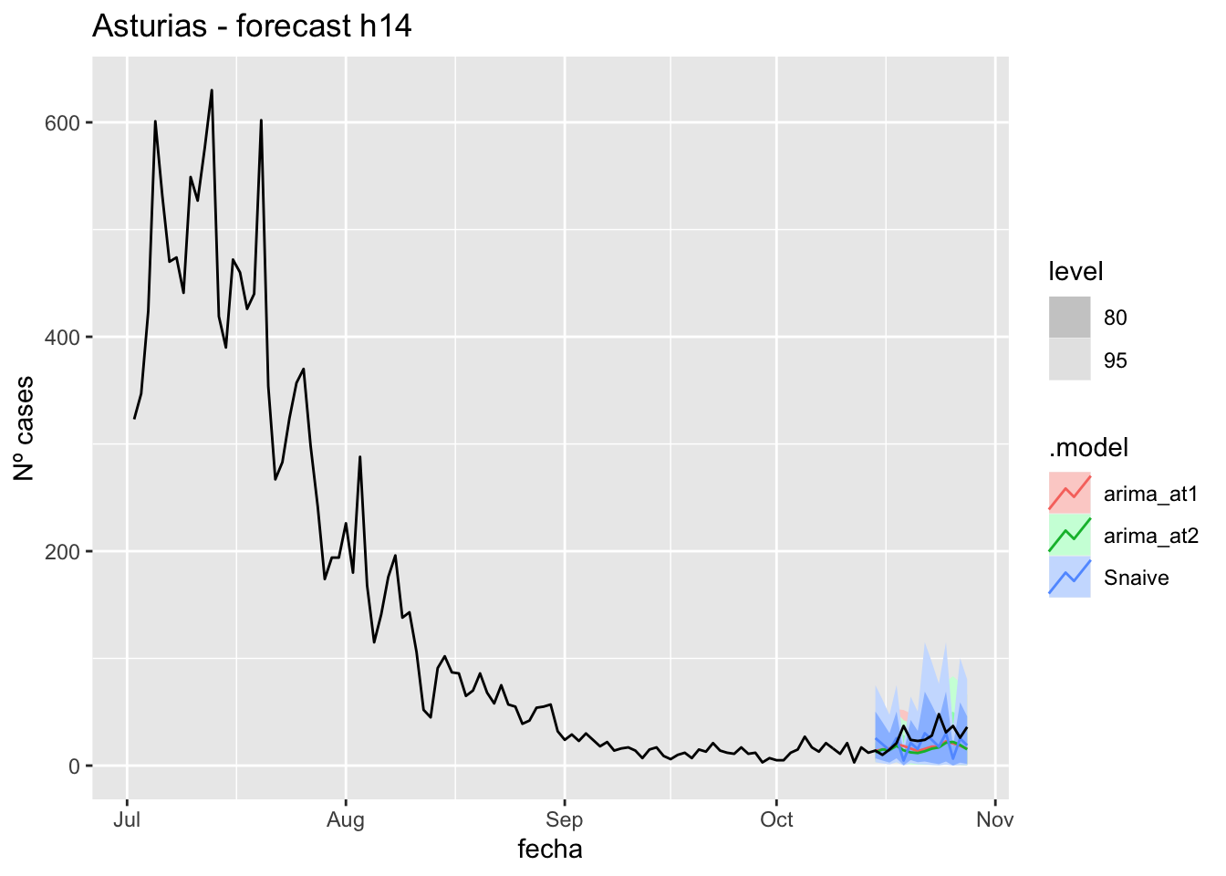
# Accuracy
fabletools::accuracy(fc_h14, data_asturias)
# A tibble: 3 × 11
.model provincia .type ME RMSE MAE MPE MAPE MASE RMSSE ACF1
<chr> <chr> <chr> <dbl> <dbl> <dbl> <dbl> <dbl> <dbl> <dbl> <dbl>
1 arima_at1 Asturias Test 9.45 13.1 10.3 26.0 34.2 0.208 0.160 0.206
2 arima_at2 Asturias Test 10.8 14.2 11.5 31.6 38.9 0.232 0.173 0.207
3 Snaive Asturias Test 6.74 15.9 11.4 8.44 41.4 0.229 0.194 -0.15121 days
# Plots
fc_h21 %>%
      autoplot(
            data_asturias_test %>%
                  filter(fecha <= as.Date("2021-10-14", format = "%Y-%m-%d")+days(21))
      ) +
      labs(y = "Nº cases", title = "Asturias - forecast h21")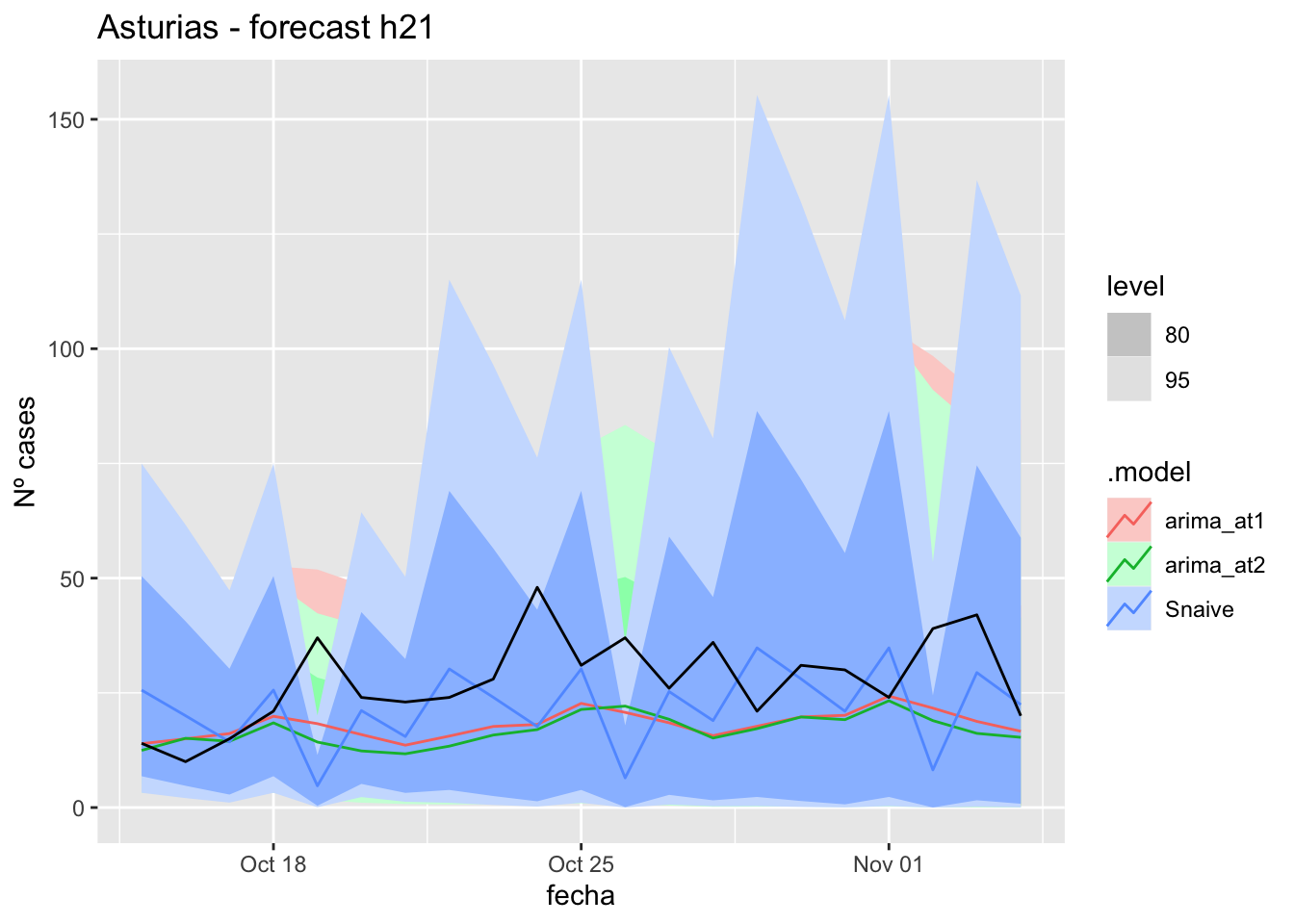
fc_h21 %>%
      autoplot(
            data_asturias %>%
                  filter(fecha <= as.Date("2021-10-14", format = "%Y-%m-%d")+days(21) &
                               fecha > as.Date("2021-07-01", format = "%Y-%m-%d"))
      ) +
      labs(y = "Nº cases", title = "Asturias - forecast h21")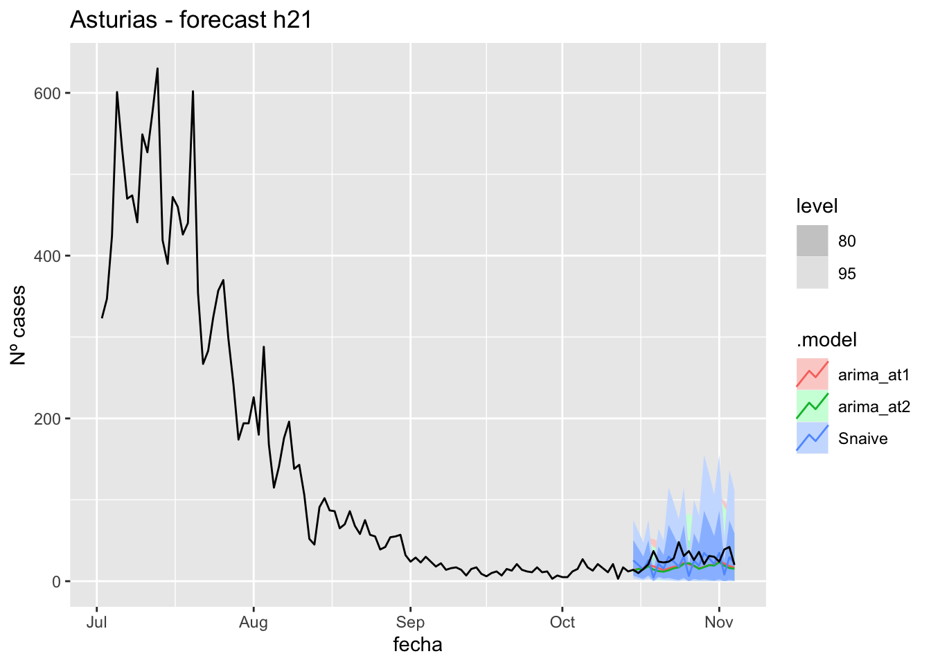
# Accuracy
fabletools::accuracy(fc_h21, data_asturias)
# A tibble: 3 × 11
.model provincia .type ME RMSE MAE MPE MAPE MASE RMSSE ACF1
<chr> <chr> <chr> <dbl> <dbl> <dbl> <dbl> <dbl> <dbl> <dbl> <dbl>
1 arima_at1 Asturias Test 9.54 12.9 10.2 26.9 32.5 0.204 0.157 0.0649
2 arima_at2 Asturias Test 10.9 14.1 11.4 32.0 36.9 0.229 0.172 0.0752
3 Snaive Asturias Test 5.84 15.5 11.5 6.84 40.5 0.231 0.189 -0.218 90 days
# Plots
fc_h90 %>%
      autoplot(
            data_asturias_test %>%
                  filter(fecha <= as.Date("2021-10-14", format = "%Y-%m-%d")+days(90))
      ) +
      labs(y = "Nº cases", title = "Asturias - forecast h90")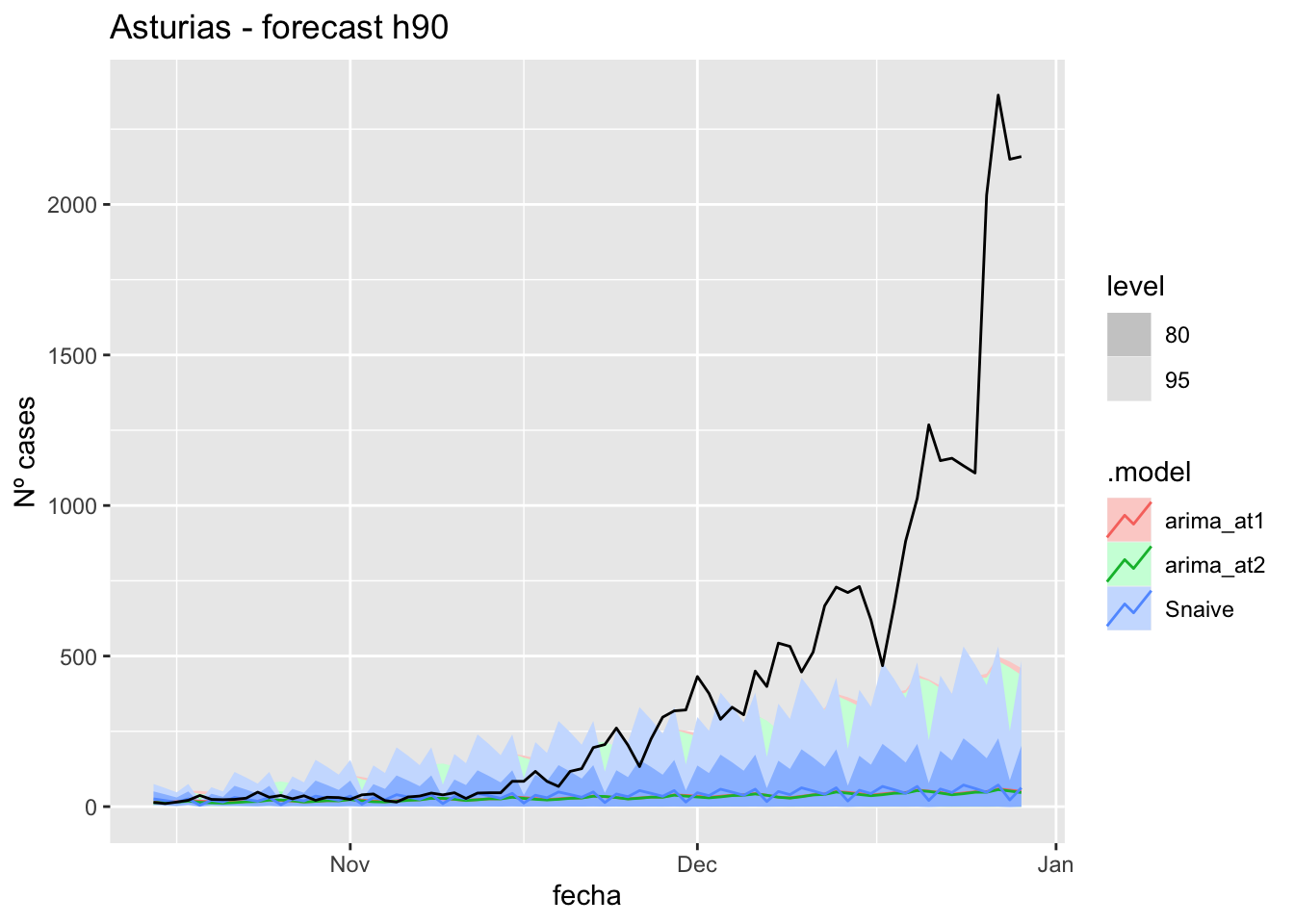
fc_h90 %>%
      autoplot(
            data_asturias %>%
                  filter(fecha <= as.Date("2021-10-14", format = "%Y-%m-%d")+days(90) &
                               fecha > as.Date("2021-07-01", format = "%Y-%m-%d"))
      ) +
      labs(y = "Nº cases", title = "Asturias - forecast h90")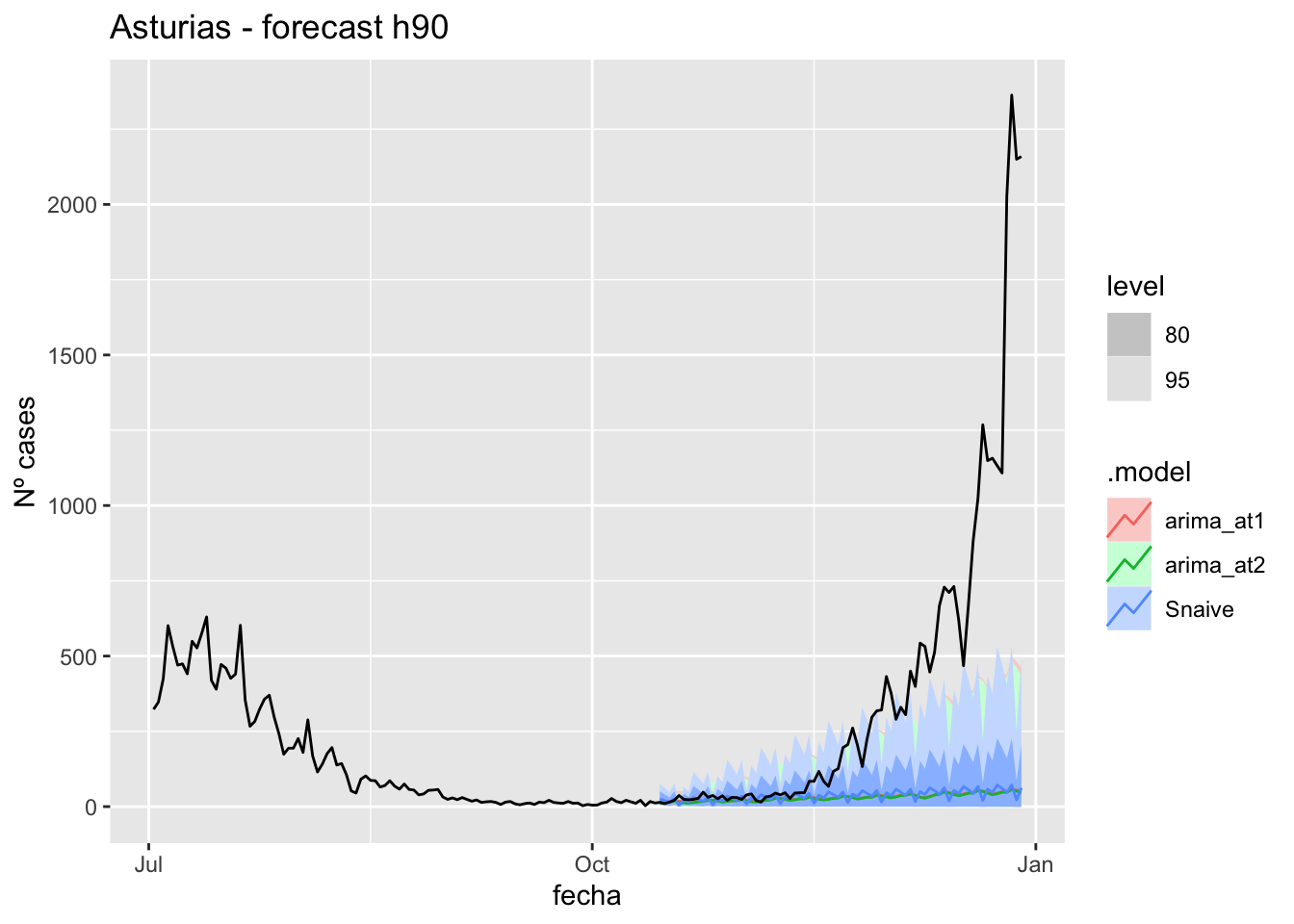
# Accuracy
fabletools::accuracy(fc_h90, data_asturias)
# A tibble: 3 × 11
.model provincia .type ME RMSE MAE MPE MAPE MASE RMSSE ACF1
<chr> <chr> <chr> <dbl> <dbl> <dbl> <dbl> <dbl> <dbl> <dbl> <dbl>
1 arima_at1 Asturias Test 356. 636. 356. 63.8 66.1 7.17 7.76 0.892
2 arima_at2 Asturias Test 358. 638. 358. 65.8 67.6 7.20 7.77 0.892
3 Snaive Asturias Test 351. 635. 353. 53.3 66.9 7.10 7.74 0.892Barcelona
data_Barcelona <- covid_data %>%
      filter(provincia == "Barcelona") %>%
      filter(fecha > as.Date("2020-06-14", format = "%Y-%m-%d")) %>%
      select(provincia, fecha, num_casos, tmed, mob_flujo) %>%
      drop_na() %>%
      as_tsibble(key = provincia, index = fecha)
data_Barcelona
# A tsibble: 563 x 5 [1D]
# Key: provincia [1]
provincia fecha num_casos tmed mob_flujo
<chr> <date> <dbl> <dbl> <dbl>
1 Barcelona 2020-06-15 62 21.2 22.0
2 Barcelona 2020-06-16 66 20.8 22.6
3 Barcelona 2020-06-17 70 20.3 23.2
4 Barcelona 2020-06-18 68 18.8 23.2
5 Barcelona 2020-06-19 65 20.4 23.9
6 Barcelona 2020-06-20 53 21.8 21.5
7 Barcelona 2020-06-21 38 22.8 20.5
8 Barcelona 2020-06-22 69 23.8 19.5
9 Barcelona 2020-06-23 95 23.4 18.5
10 Barcelona 2020-06-24 44 23.6 17.5
# … with 553 more rowsdata_Barcelona_train <- data_Barcelona %>%
filter(fecha <= as.Date("2021-10-14", format = "%Y-%m-%d"))
summary(data_Barcelona_train$fecha) Min. 1st Qu. Median Mean 3rd Qu. Max.
"2020-06-15" "2020-10-14" "2021-02-13" "2021-02-13" "2021-06-14" "2021-10-14" data_Barcelona_test <- data_Barcelona %>%
filter(fecha > as.Date("2021-10-14", format = "%Y-%m-%d"))
summary(data_Barcelona_test$fecha) Min. 1st Qu. Median Mean 3rd Qu. Max.
"2021-10-15" "2021-11-02" "2021-11-21" "2021-11-21" "2021-12-10" "2021-12-29" # Lamba for num_casos
lambda_Barcelona_casos <- data_Barcelona %>%
features(num_casos, features = guerrero) %>%
pull(lambda_guerrero)
lambda_Barcelona_casos[1] 0.07878312# Lamba for average temp
lambda_Barcelona_tmed <- data_Barcelona %>%
features(tmed, features = guerrero) %>%
pull(lambda_guerrero)
lambda_Barcelona_tmed[1] 1.143918# Lamba for mobility
lambda_Barcelona_mobil <- data_Barcelona %>%
features(mob_flujo, features = guerrero) %>%
pull(lambda_guerrero)
lambda_Barcelona_mobil[1] 1.072959fit_model <- data_Barcelona_train %>%
model(
arima_at1 = ARIMA(box_cox(num_casos, lambda_Barcelona_casos) ~
box_cox(tmed, lambda_Barcelona_tmed) +
box_cox(mob_flujo, lambda_Barcelona_mobil)),
arima_at2 = ARIMA(box_cox(num_casos, lambda_Barcelona_casos) ~
box_cox(tmed, lambda_Barcelona_tmed) +
box_cox(mob_flujo, lambda_Barcelona_mobil),
stepwise = FALSE, approx = FALSE),
Snaive = SNAIVE(box_cox(num_casos, lambda_Barcelona_casos))
)
# Show and report model
fit_model# A mable: 1 x 4
# Key: provincia [1]
provincia arima_at1
<chr> <model>
1 Barcelona <LM w/ ARIMA(1,1,2)(1,1,2)[7] errors>
# … with 2 more variables: arima_at2 <model>, Snaive <model>glance(fit_model)# A tibble: 3 × 9
provincia .model sigma2 log_lik AIC AICc BIC ar_roots ma_roots
<chr> <chr> <dbl> <dbl> <dbl> <dbl> <dbl> <list> <list>
1 Barcelona arima_at1 0.0757 -63.1 144. 145. 182. <cpl [8]> <cpl [16]>
2 Barcelona arima_at2 0.0756 -63.3 143. 143. 176. <cpl [8]> <cpl [9]>
3 Barcelona Snaive 0.389 NA NA NA NA <NULL> <NULL> fit_model %>%
pivot_longer(-provincia,
names_to = ".model",
values_to = "orders") %>%
left_join(glance(fit_model), by = c("provincia", ".model")) %>%
arrange(AICc) %>%
select(.model:BIC)# A mable: 3 x 7
# Key: .model [3]
.model orders sigma2 log_lik AIC AICc BIC
<chr> <model> <dbl> <dbl> <dbl> <dbl> <dbl>
1 arima_… <LM w/ ARIMA(1,1,2)(1,1,1)[7] errors> 0.0756 -63.3 143. 143. 176.
2 arima_… <LM w/ ARIMA(1,1,2)(1,1,2)[7] errors> 0.0757 -63.1 144. 145. 182.
3 Snaive <SNAIVE> 0.389 NA NA NA NA # We use a Ljung-Box test >> large p-value, confirms residuals are similar / considered to white noise
fit_model %>%
select(Snaive) %>%
gg_tsresiduals()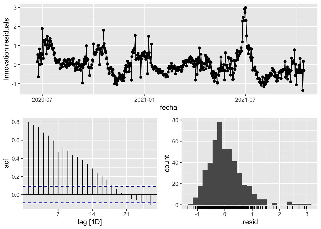
fit_model %>%
      select(arima_at1) %>%
      gg_tsresiduals()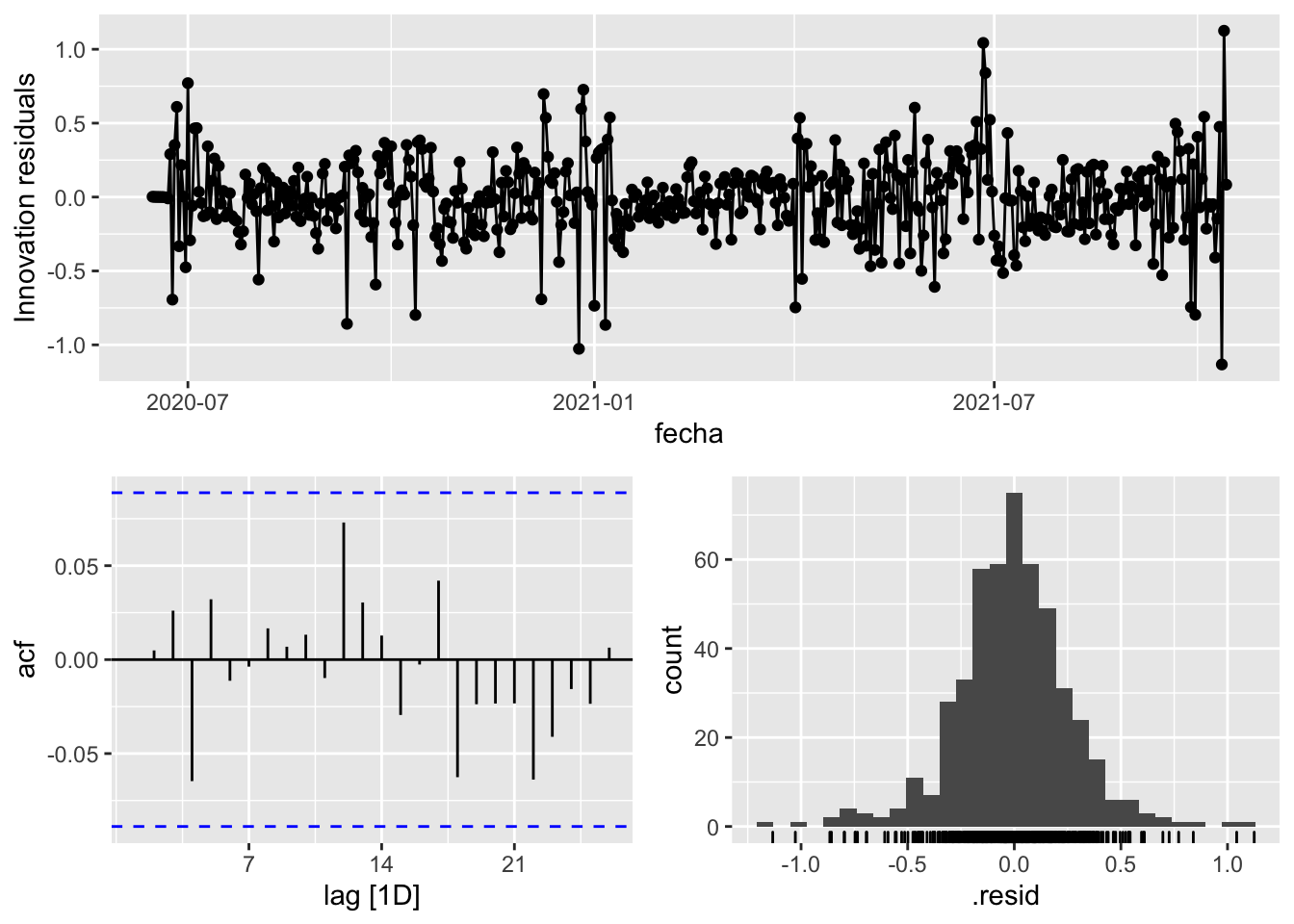
fit_model %>%
      select(arima_at2) %>%
      gg_tsresiduals()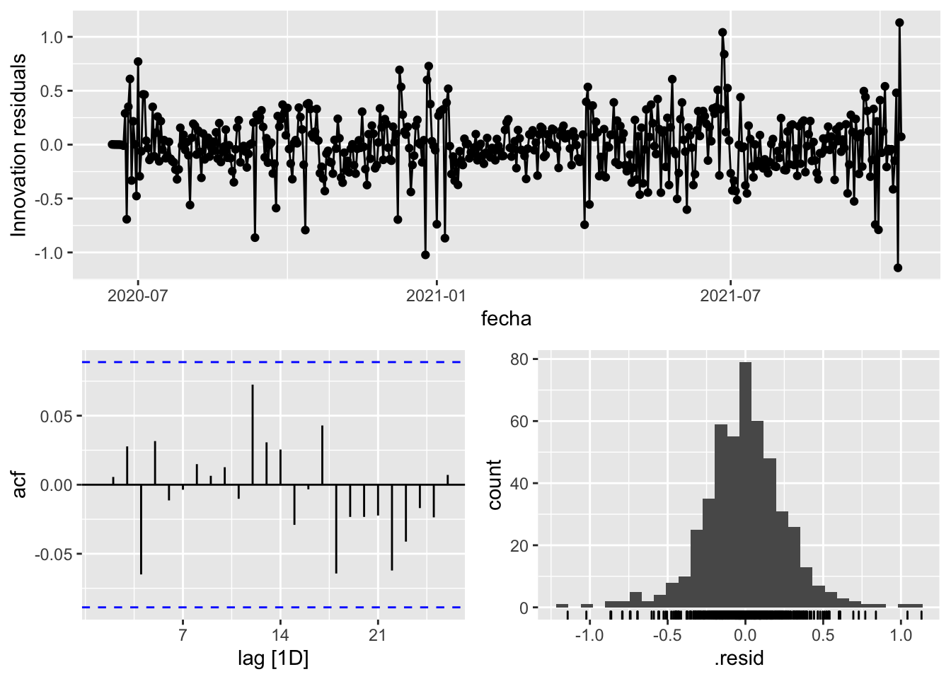
augment(fit_model) %>%
      features(.innov, ljung_box, lag=7)
# A tibble: 3 × 4
provincia .model lb_stat lb_pvalue
<chr> <chr> <dbl> <dbl>
1 Barcelona arima_at1 2.99 0.886
2 Barcelona arima_at2 3.04 0.881
3 Barcelona Snaive 1575. 0 augment(fit_model) %>%
features(.innov, ljung_box, lag=14)# A tibble: 3 × 4
provincia .model lb_stat lb_pvalue
<chr> <chr> <dbl> <dbl>
1 Barcelona arima_at1 6.50 0.952
2 Barcelona arima_at2 6.74 0.944
3 Barcelona Snaive 2173. 0 augment(fit_model) %>%
features(.innov, ljung_box, lag=21)# A tibble: 3 × 4
provincia .model lb_stat lb_pvalue
<chr> <chr> <dbl> <dbl>
1 Barcelona arima_at1 10.7 0.969
2 Barcelona arima_at2 11.0 0.963
3 Barcelona Snaive 2244. 0 augment(fit_model) %>%
features(.innov, ljung_box, lag=90)# A tibble: 3 × 4
provincia .model lb_stat lb_pvalue
<chr> <chr> <dbl> <dbl>
1 Barcelona arima_at1 77.9 0.814
2 Barcelona arima_at2 78.3 0.805
3 Barcelona Snaive 3329. 0 # To predict future values of infections, we need to pass the model future/prediction values of the complementary variables tmed and mobility
# We are going to select those from the test dataset
data_fc_h7 <- data_Barcelona_test %>%
select(-num_casos) %>%
slice(1:7)
data_fc_h14 <- data_Barcelona_test %>%
select(-num_casos) %>%
slice(1:14)
data_fc_h21 <- data_Barcelona_test %>%
select(-num_casos) %>%
slice(1:21)
data_fc_h90 <- data_Barcelona_test %>%
select(-num_casos) %>%
slice(1:90)# Significant spikes out of 30 is still consistent with white noise
# To be sure, use a Ljung-Box test, which has a large p-value, confirming that
# the residuals are similar to white noise.
# Note that the alternative models also passed this test.
#
# Forecast
fc_h7 <- fabletools::forecast(fit_model, new_data = data_fc_h7)
fc_h14 <- fabletools::forecast(fit_model, new_data = data_fc_h14)
fc_h21 <- fabletools::forecast(fit_model, new_data = data_fc_h21)
fc_h90 <- fabletools::forecast(fit_model, new_data = data_fc_h90)7 days
# Plots
fc_h7 %>%
      autoplot(
            data_Barcelona_test %>%
                  filter(fecha <= as.Date("2021-10-14", format = "%Y-%m-%d")+days(7))
      ) +
      labs(y = "Nº cases", title = "Barcelona - forecast h7")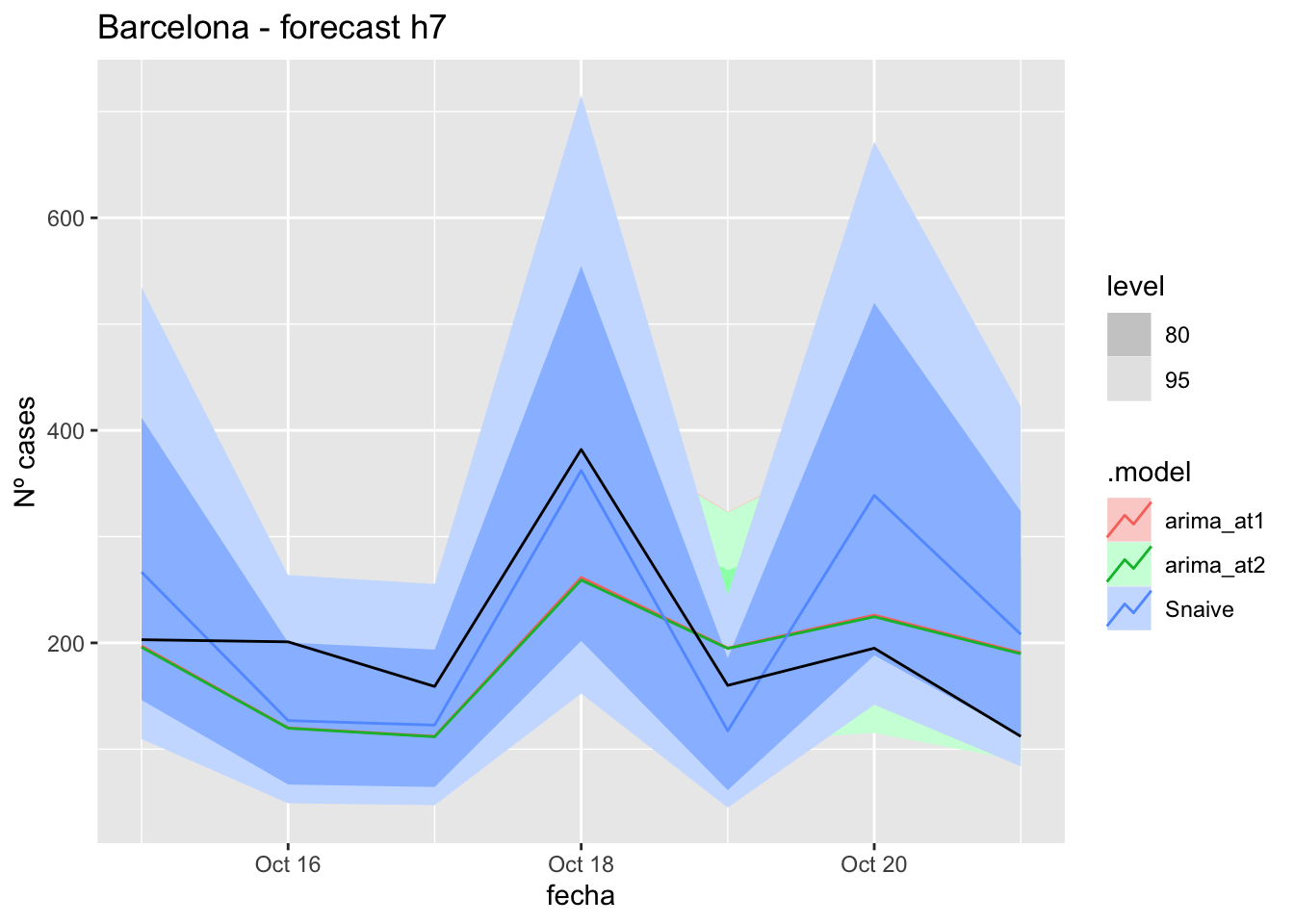
fc_h7 %>%
      autoplot(
            data_Barcelona %>%
                  filter(fecha <= as.Date("2021-10-14", format = "%Y-%m-%d")+days(7) &
                               fecha > as.Date("2021-07-01", format = "%Y-%m-%d"))
      ) +
      labs(y = "Nº cases", title = "Barcelona - forecast h7")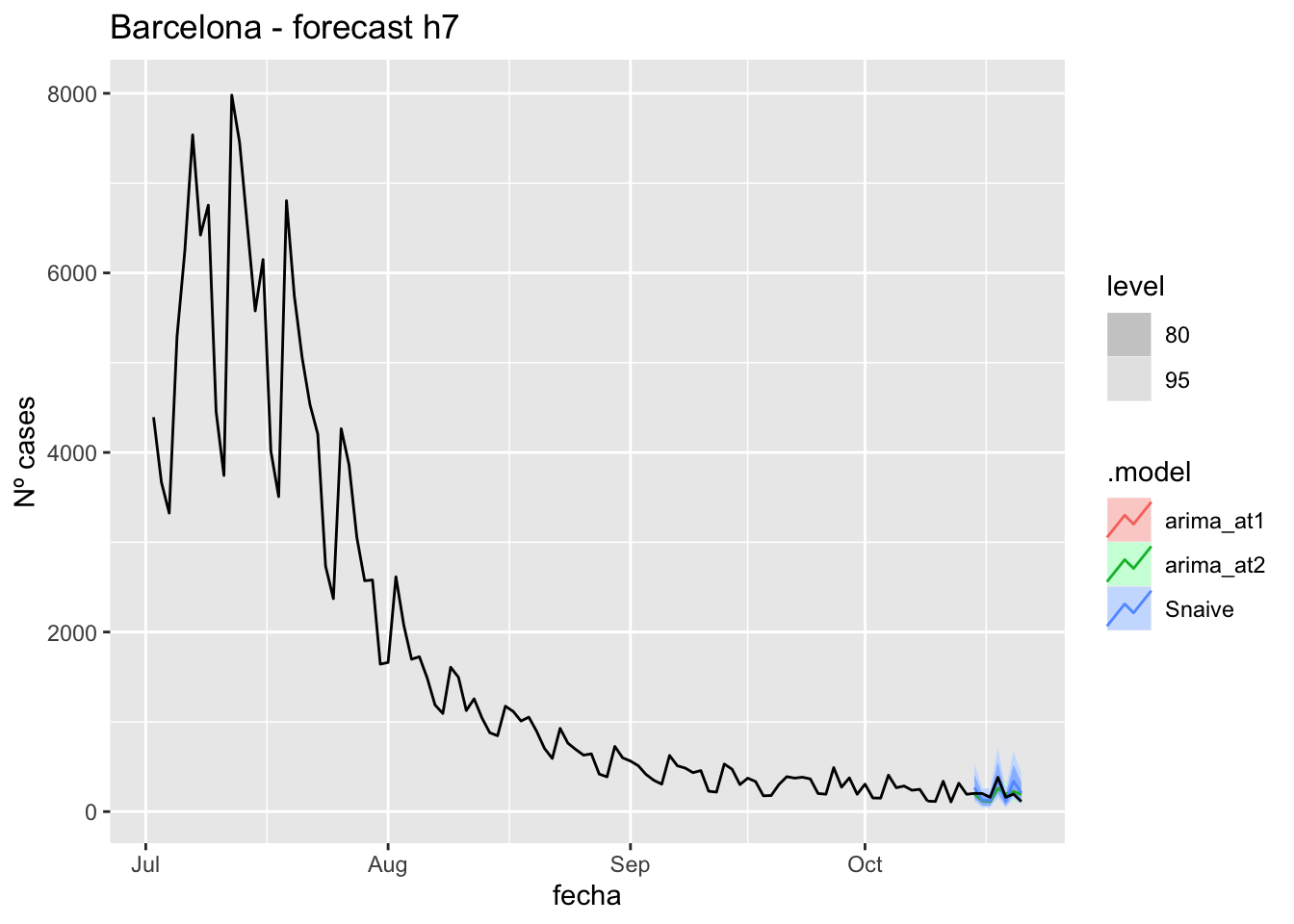
# Accuracy
fabletools::accuracy(fc_h7, data_Barcelona)
# A tibble: 3 × 11
.model provincia .type ME RMSE MAE MPE MAPE MASE RMSSE ACF1
<chr> <chr> <chr> <dbl> <dbl> <dbl> <dbl> <dbl> <dbl> <dbl> <dbl>
1 arima_at1 Barcelona Test 15.6 67.3 57.0 -0.568 30.3 0.152 0.101 0.206
2 arima_at2 Barcelona Test 16.6 67.7 57.2 -0.0595 30.3 0.152 0.102 0.195
3 Snaive Barcelona Test -18.6 78.4 68.1 -14.2 40.4 0.181 0.118 0.18314 days
# Plots
fc_h14 %>%
      autoplot(
            data_Barcelona_test %>%
                  filter(fecha <= as.Date("2021-10-14", format = "%Y-%m-%d")+days(14))
      ) +
      labs(y = "Nº cases", title = "Barcelona - forecast h14")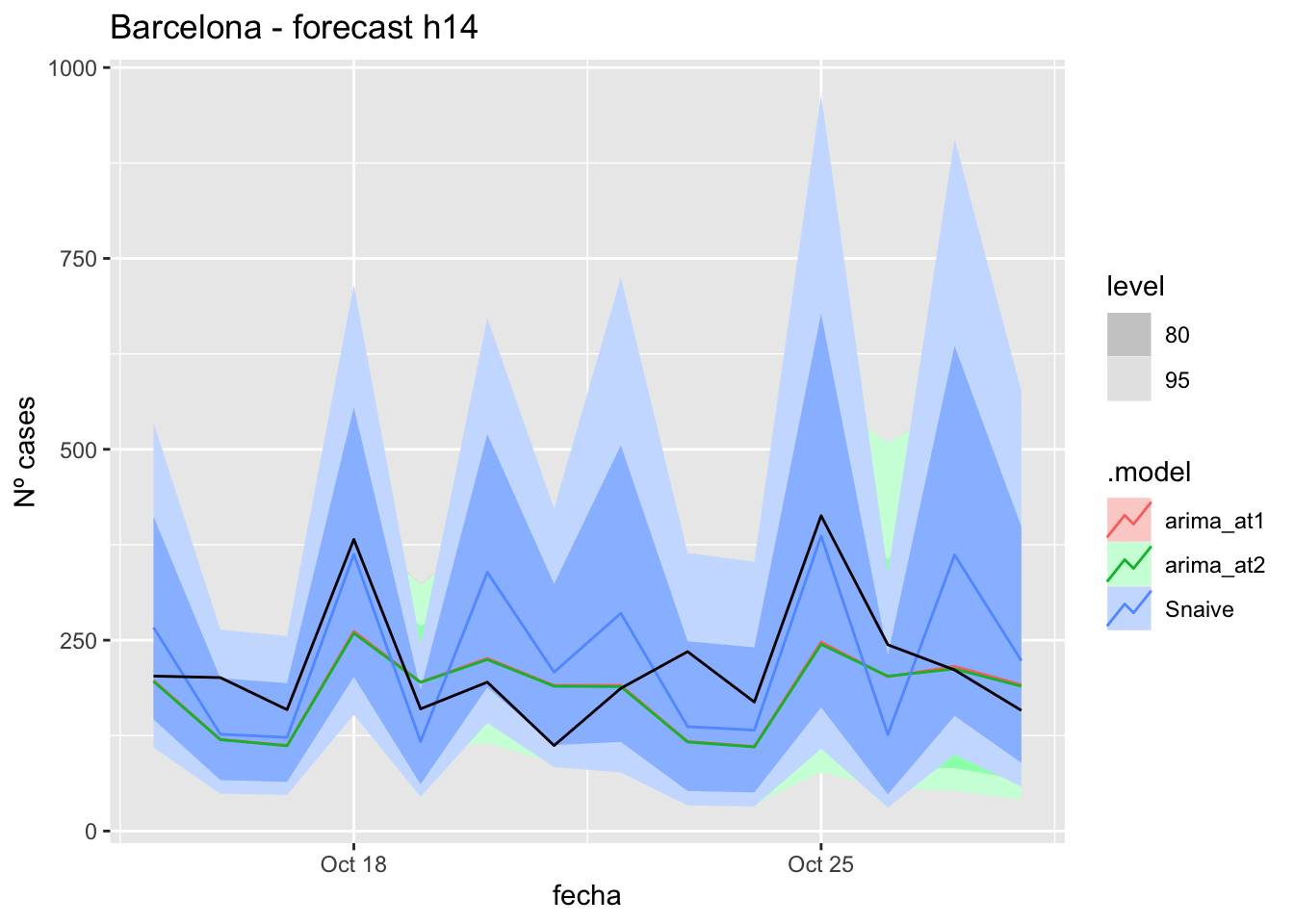
fc_h14 %>%
      autoplot(
            data_Barcelona %>%
                  filter(fecha <= as.Date("2021-10-14", format = "%Y-%m-%d")+days(14) &
                               fecha > as.Date("2021-07-01", format = "%Y-%m-%d"))
      ) +
      labs(y = "Nº cases", title = "Barcelona - forecast h14")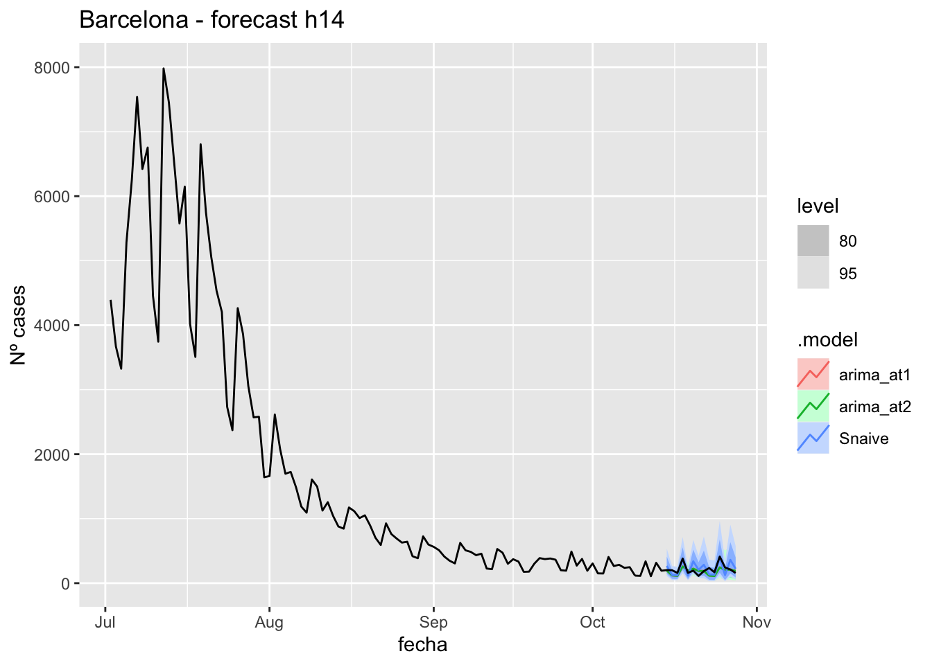
# Accuracy
fabletools::accuracy(fc_h14, data_Barcelona)
# A tibble: 3 × 11
.model provincia .type ME RMSE MAE MPE MAPE MASE RMSSE ACF1
<chr> <chr> <chr> <dbl> <dbl> <dbl> <dbl> <dbl> <dbl> <dbl> <dbl>
1 arima_at1 Barcelona Test 32.2 75.2 58.9 8.01 27.1 0.156 0.113 0.248
2 arima_at2 Barcelona Test 33.4 75.9 58.8 8.61 26.9 0.156 0.114 0.237
3 Snaive Barcelona Test -11.8 86.7 76.4 -10.4 40.4 0.203 0.131 0.060821 days
# Plots
fc_h21 %>%
      autoplot(
            data_Barcelona_test %>%
                  filter(fecha <= as.Date("2021-10-14", format = "%Y-%m-%d")+days(21))
      ) +
      labs(y = "Nº cases", title = "Barcelona - forecast h21")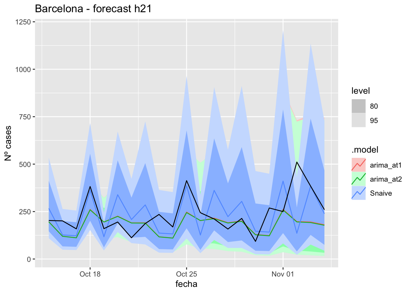
fc_h21 %>%
      autoplot(
            data_Barcelona %>%
                  filter(fecha <= as.Date("2021-10-14", format = "%Y-%m-%d")+days(21) &
                               fecha > as.Date("2021-07-01", format = "%Y-%m-%d"))
      ) +
      labs(y = "Nº cases", title = "Barcelona - forecast h21")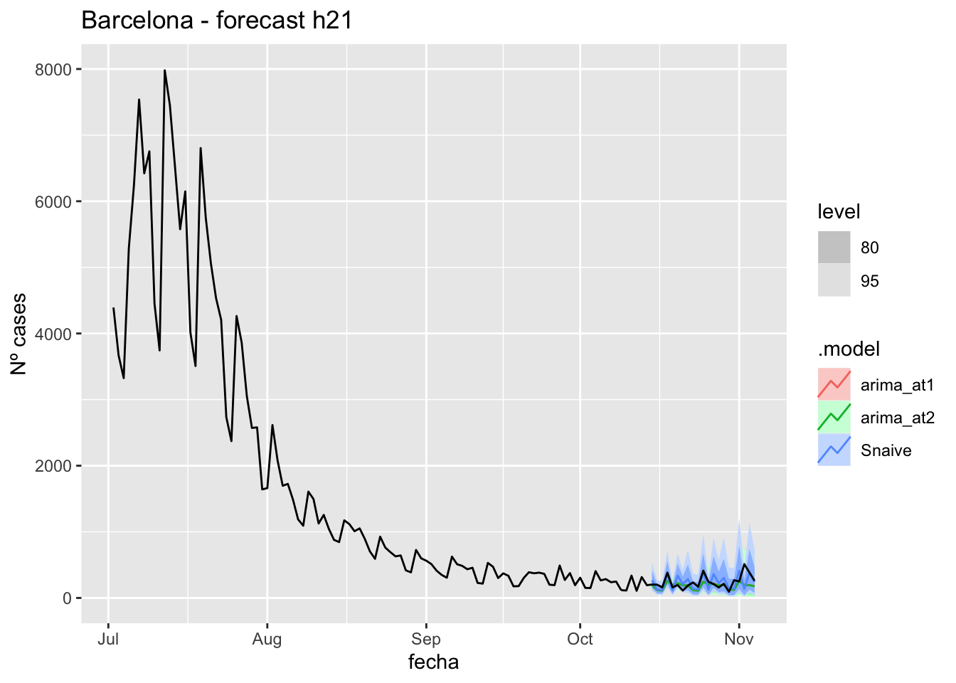
# Accuracy
fabletools::accuracy(fc_h21, data_Barcelona)
# A tibble: 3 × 11
.model provincia .type ME RMSE MAE MPE MAPE MASE RMSSE ACF1
<chr> <chr> <chr> <dbl> <dbl> <dbl> <dbl> <dbl> <dbl> <dbl> <dbl>
1 arima_at1 Barcelona Test 54.4 107. 76.8 12.9 29.7 0.204 0.162 0.193
2 arima_at2 Barcelona Test 56.1 108. 77.0 13.6 29.6 0.205 0.164 0.196
3 Snaive Barcelona Test 2.57 119. 90.4 -8.63 40.9 0.240 0.180 -0.23590 days
# Plots
fc_h90 %>%
      autoplot(
            data_Barcelona_test %>%
                  filter(fecha <= as.Date("2021-10-14", format = "%Y-%m-%d")+days(90))
      ) +
      labs(y = "Nº cases", title = "Barcelona - forecast h90")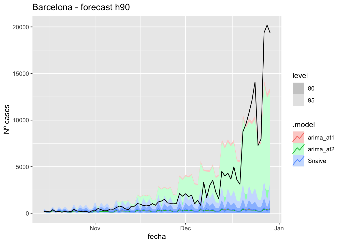
fc_h90 %>%
      autoplot(
            data_Barcelona %>%
                  filter(fecha <= as.Date("2021-10-14", format = "%Y-%m-%d")+days(90) &
                               fecha > as.Date("2021-07-01", format = "%Y-%m-%d"))
      ) +
      labs(y = "Nº cases", title = "Barcelona - forecast h90")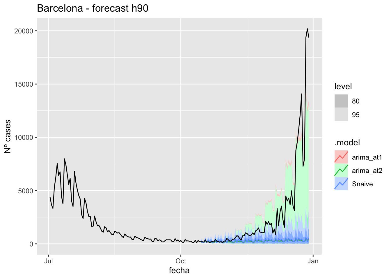
# Accuracy
fabletools::accuracy(fc_h90, data_Barcelona)
# A tibble: 3 × 11
.model provincia .type ME RMSE MAE MPE MAPE MASE RMSSE ACF1
<chr> <chr> <chr> <dbl> <dbl> <dbl> <dbl> <dbl> <dbl> <dbl> <dbl>
1 arima_at1 Barcelona Test 2529. 5090. 2535. 62.2 66.8 6.73 7.68 0.827
2 arima_at2 Barcelona Test 2536. 5098. 2542. 62.8 67.2 6.75 7.69 0.827
3 Snaive Barcelona Test 2482. 5070. 2508. 53.0 67.2 6.66 7.65 0.829Madrid
data_Madrid <- covid_data %>%
      filter(provincia == "Madrid") %>%
      filter(fecha > as.Date("2020-06-14", format = "%Y-%m-%d")) %>%
      select(provincia, fecha, num_casos, tmed, mob_flujo) %>%
      drop_na() %>%
      as_tsibble(key = provincia, index = fecha)
data_Madrid
# A tsibble: 563 x 5 [1D]
# Key: provincia [1]
provincia fecha num_casos tmed mob_flujo
<chr> <date> <dbl> <dbl> <dbl>
1 Madrid 2020-06-15 153 20.7 20.6
2 Madrid 2020-06-16 91 21 21.6
3 Madrid 2020-06-17 93 20.2 21.8
4 Madrid 2020-06-18 85 21.9 22.1
5 Madrid 2020-06-19 78 22.6 22.0
6 Madrid 2020-06-20 67 23.4 18.8
7 Madrid 2020-06-21 42 25 19.9
8 Madrid 2020-06-22 60 27.3 21.0
9 Madrid 2020-06-23 68 28.4 22.1
10 Madrid 2020-06-24 49 28 23.1
# … with 553 more rowsdata_Madrid_train <- data_Madrid %>%
filter(fecha <= as.Date("2021-10-14", format = "%Y-%m-%d"))
summary(data_Madrid_train$fecha) Min. 1st Qu. Median Mean 3rd Qu. Max.
"2020-06-15" "2020-10-14" "2021-02-13" "2021-02-13" "2021-06-14" "2021-10-14" data_Madrid_test <- data_Madrid %>%
filter(fecha > as.Date("2021-10-14", format = "%Y-%m-%d"))
summary(data_Madrid_test$fecha) Min. 1st Qu. Median Mean 3rd Qu. Max.
"2021-10-15" "2021-11-02" "2021-11-21" "2021-11-21" "2021-12-10" "2021-12-29" # Lamba for num_casos
lambda_Madrid_casos <- data_Madrid %>%
features(num_casos, features = guerrero) %>%
pull(lambda_guerrero)
lambda_Madrid_casos[1] 0.004154257# Lamba for average temp
lambda_Madrid_tmed <- data_Madrid %>%
features(tmed, features = guerrero) %>%
pull(lambda_guerrero)
lambda_Madrid_tmed[1] 0.9461578# Lamba for mobility
lambda_Madrid_mobil <- data_Madrid %>%
features(mob_flujo, features = guerrero) %>%
pull(lambda_guerrero)
lambda_Madrid_mobil[1] -0.01895186fit_model <- data_Madrid_train %>%
model(
arima_at1 = ARIMA(box_cox(num_casos, lambda_Madrid_casos) ~
box_cox(tmed, lambda_Madrid_tmed) +
box_cox(mob_flujo, lambda_Madrid_mobil)),
arima_at2 = ARIMA(box_cox(num_casos, lambda_Madrid_casos) ~
box_cox(tmed, lambda_Madrid_tmed) +
box_cox(mob_flujo, lambda_Madrid_mobil),
stepwise = FALSE, approx = FALSE),
Snaive = SNAIVE(box_cox(num_casos, lambda_Madrid_casos))
)
# Show and report model
fit_model# A mable: 1 x 4
# Key: provincia [1]
provincia arima_at1
<chr> <model>
1 Madrid <LM w/ ARIMA(2,1,1)(1,1,1)[7] errors>
# … with 2 more variables: arima_at2 <model>, Snaive <model>glance(fit_model)# A tibble: 3 × 9
provincia .model sigma2 log_lik AIC AICc BIC ar_roots ma_roots
<chr> <chr> <dbl> <dbl> <dbl> <dbl> <dbl> <list> <list>
1 Madrid arima_at1 0.0295 164. -311. -311. -278. <cpl [9]> <cpl [8]>
2 Madrid arima_at2 0.0293 166. -314. -314. -276. <cpl [3]> <cpl [15]>
3 Madrid Snaive 0.131 NA NA NA NA <NULL> <NULL> fit_model %>%
pivot_longer(-provincia,
names_to = ".model",
values_to = "orders") %>%
left_join(glance(fit_model), by = c("provincia", ".model")) %>%
arrange(AICc) %>%
select(.model:BIC)# A mable: 3 x 7
# Key: .model [3]
.model orders sigma2 log_lik AIC AICc BIC
<chr> <model> <dbl> <dbl> <dbl> <dbl> <dbl>
1 arima_… <LM w/ ARIMA(3,1,1)(0,1,2)[7] errors> 0.0293 166. -314. -314. -276.
2 arima_… <LM w/ ARIMA(2,1,1)(1,1,1)[7] errors> 0.0295 164. -311. -311. -278.
3 Snaive <SNAIVE> 0.131 NA NA NA NA # We use a Ljung-Box test >> large p-value, confirms residuals are similar / considered to white noise
fit_model %>%
select(Snaive) %>%
gg_tsresiduals()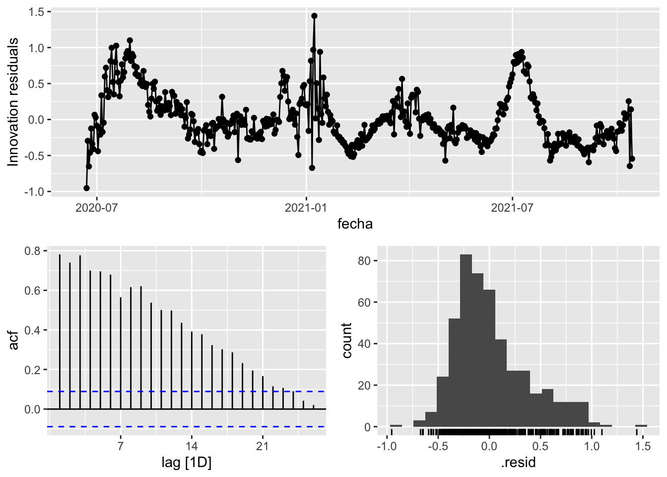
fit_model %>%
      select(arima_at1) %>%
      gg_tsresiduals()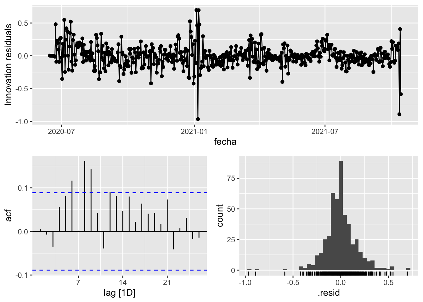
fit_model %>%
      select(arima_at2) %>%
      gg_tsresiduals()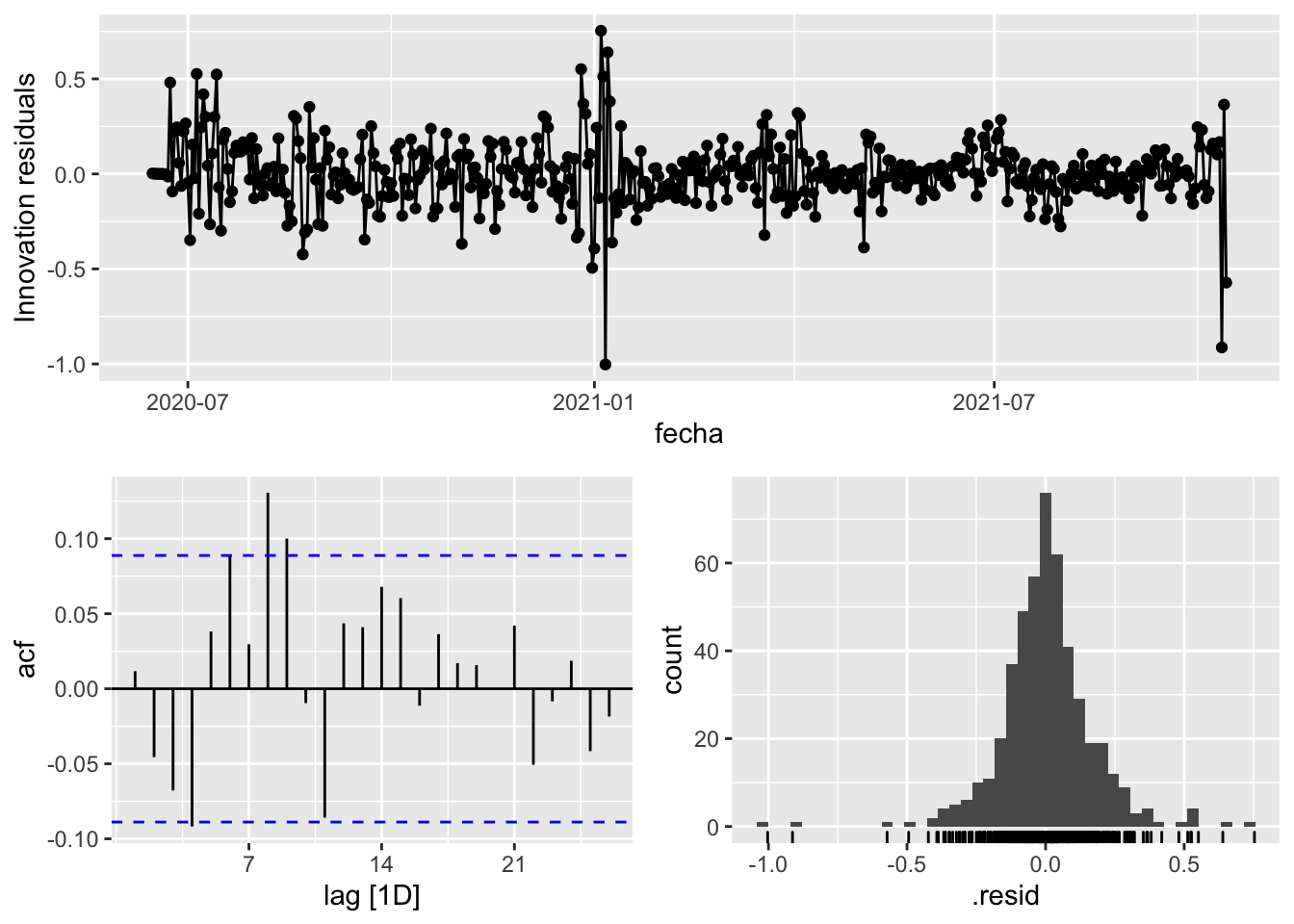
augment(fit_model) %>%
      features(.innov, ljung_box, lag=7)
# A tibble: 3 × 4
provincia .model lb_stat lb_pvalue
<chr> <chr> <dbl> <dbl>
1 Madrid arima_at1 12.2 0.0943
2 Madrid arima_at2 12.6 0.0826
3 Madrid Snaive 1708. 0 augment(fit_model) %>%
features(.innov, ljung_box, lag=14)# A tibble: 3 × 4
provincia .model lb_stat lb_pvalue
<chr> <chr> <dbl> <dbl>
1 Madrid arima_at1 45.5 0.0000344
2 Madrid arima_at2 33.9 0.00211
3 Madrid Snaive 2642. 0 augment(fit_model) %>%
features(.innov, ljung_box, lag=21)# A tibble: 3 × 4
provincia .model lb_stat lb_pvalue
<chr> <chr> <dbl> <dbl>
1 Madrid arima_at1 55.6 0.0000574
2 Madrid arima_at2 37.7 0.0140
3 Madrid Snaive 2912. 0 augment(fit_model) %>%
features(.innov, ljung_box, lag=90)# A tibble: 3 × 4
provincia .model lb_stat lb_pvalue
<chr> <chr> <dbl> <dbl>
1 Madrid arima_at1 111. 0.0674
2 Madrid arima_at2 91.3 0.442
3 Madrid Snaive 3833. 0 # To predict future values of infections, we need to pass the model future/prediction values of the complementary variables tmed and mobility
# We are going to select those from the test dataset
data_fc_h7 <- data_Madrid_test %>%
select(-num_casos) %>%
slice(1:7)
data_fc_h14 <- data_Madrid_test %>%
select(-num_casos) %>%
slice(1:14)
data_fc_h21 <- data_Madrid_test %>%
select(-num_casos) %>%
slice(1:21)
data_fc_h90 <- data_Madrid_test %>%
select(-num_casos) %>%
slice(1:90)# Significant spikes out of 30 is still consistent with white noise
# To be sure, use a Ljung-Box test, which has a large p-value, confirming that
# the residuals are similar to white noise.
# Note that the alternative models also passed this test.
#
# Forecast
fc_h7 <- fabletools::forecast(fit_model, new_data = data_fc_h7)
fc_h14 <- fabletools::forecast(fit_model, new_data = data_fc_h14)
fc_h21 <- fabletools::forecast(fit_model, new_data = data_fc_h21)
fc_h90 <- fabletools::forecast(fit_model, new_data = data_fc_h90)7 days
# Plots
fc_h7 %>%
      autoplot(
            data_Madrid_test %>%
                  filter(fecha <= as.Date("2021-10-14", format = "%Y-%m-%d")+days(7))
      ) +
      labs(y = "Nº cases", title = "Madrid - forecast h7")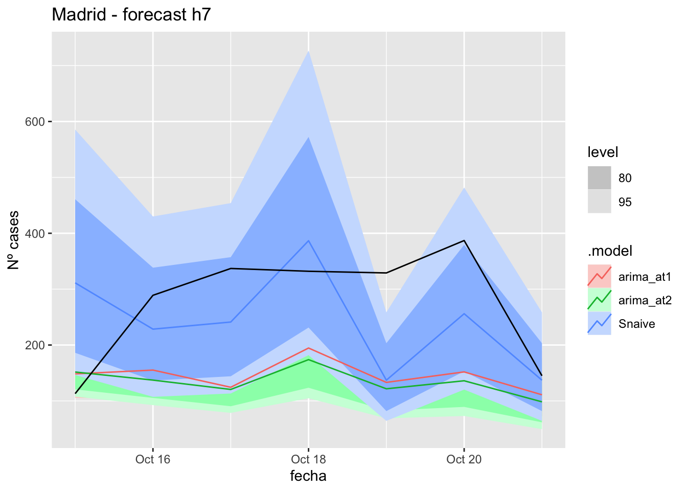
fc_h7 %>%
      autoplot(
            data_Madrid %>%
                  filter(fecha <= as.Date("2021-10-14", format = "%Y-%m-%d")+days(7) &
                               fecha > as.Date("2021-07-01", format = "%Y-%m-%d"))
      ) +
      labs(y = "Nº cases", title = "Madrid - forecast h7")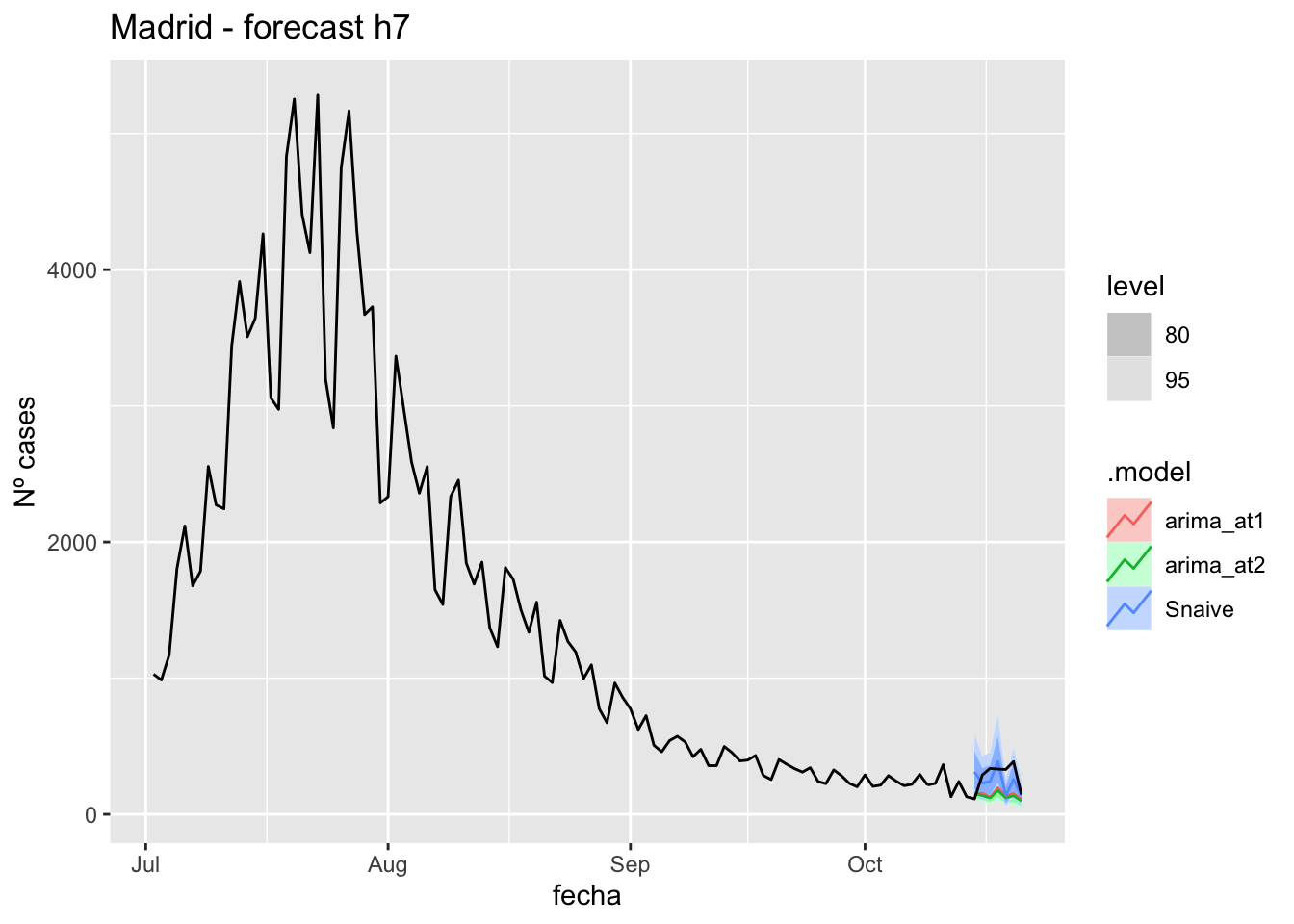
# Accuracy
fabletools::accuracy(fc_h7, data_Madrid)
# A tibble: 3 × 11
.model provincia .type ME RMSE MAE MPE MAPE MASE RMSSE ACF1
<chr> <chr> <chr> <dbl> <dbl> <dbl> <dbl> <dbl> <dbl> <dbl> <dbl>
1 arima_at1 Madrid Test 130. 159. 141. 37.6 46.5 0.331 0.237 -0.0428
2 arima_at2 Madrid Test 142. 171. 153. 41.4 51.2 0.360 0.254 -0.0313
3 Snaive Madrid Test 33.5 125. 106. -6.41 48.4 0.249 0.186 -0.109 14 days
# Plots
fc_h14 %>%
      autoplot(
            data_Madrid_test %>%
                  filter(fecha <= as.Date("2021-10-14", format = "%Y-%m-%d")+days(14))
      ) +
      labs(y = "Nº cases", title = "Madrid - forecast h14")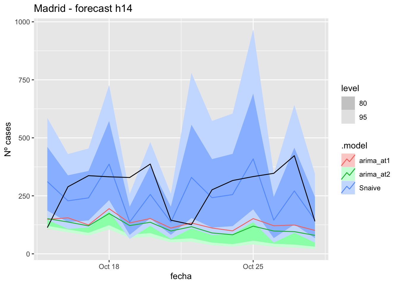
fc_h14 %>%
      autoplot(
            data_Madrid %>%
                  filter(fecha <= as.Date("2021-10-14", format = "%Y-%m-%d")+days(14) &
                               fecha > as.Date("2021-07-01", format = "%Y-%m-%d"))
      ) +
      labs(y = "Nº cases", title = "Madrid - forecast h14")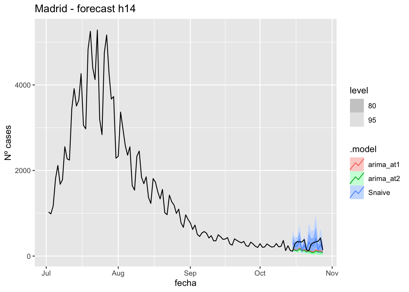
# Accuracy
fabletools::accuracy(fc_h14, data_Madrid)
# A tibble: 3 × 11
.model provincia .type ME RMSE MAE MPE MAPE MASE RMSSE ACF1
<chr> <chr> <chr> <dbl> <dbl> <dbl> <dbl> <dbl> <dbl> <dbl> <dbl>
1 arima_at1 Madrid Test 145. 175. 151. 43.2 48.4 0.357 0.260 0.0901
2 arima_at2 Madrid Test 162. 191. 168. 49.7 54.5 0.395 0.285 0.113
3 Snaive Madrid Test 28.4 127. 105. -7.67 46.6 0.248 0.189 -0.048121 days
# Plots
fc_h21 %>%
      autoplot(
            data_Madrid_test %>%
                  filter(fecha <= as.Date("2021-10-14", format = "%Y-%m-%d")+days(21))
      ) +
      labs(y = "Nº cases", title = "Madrid - forecast h21")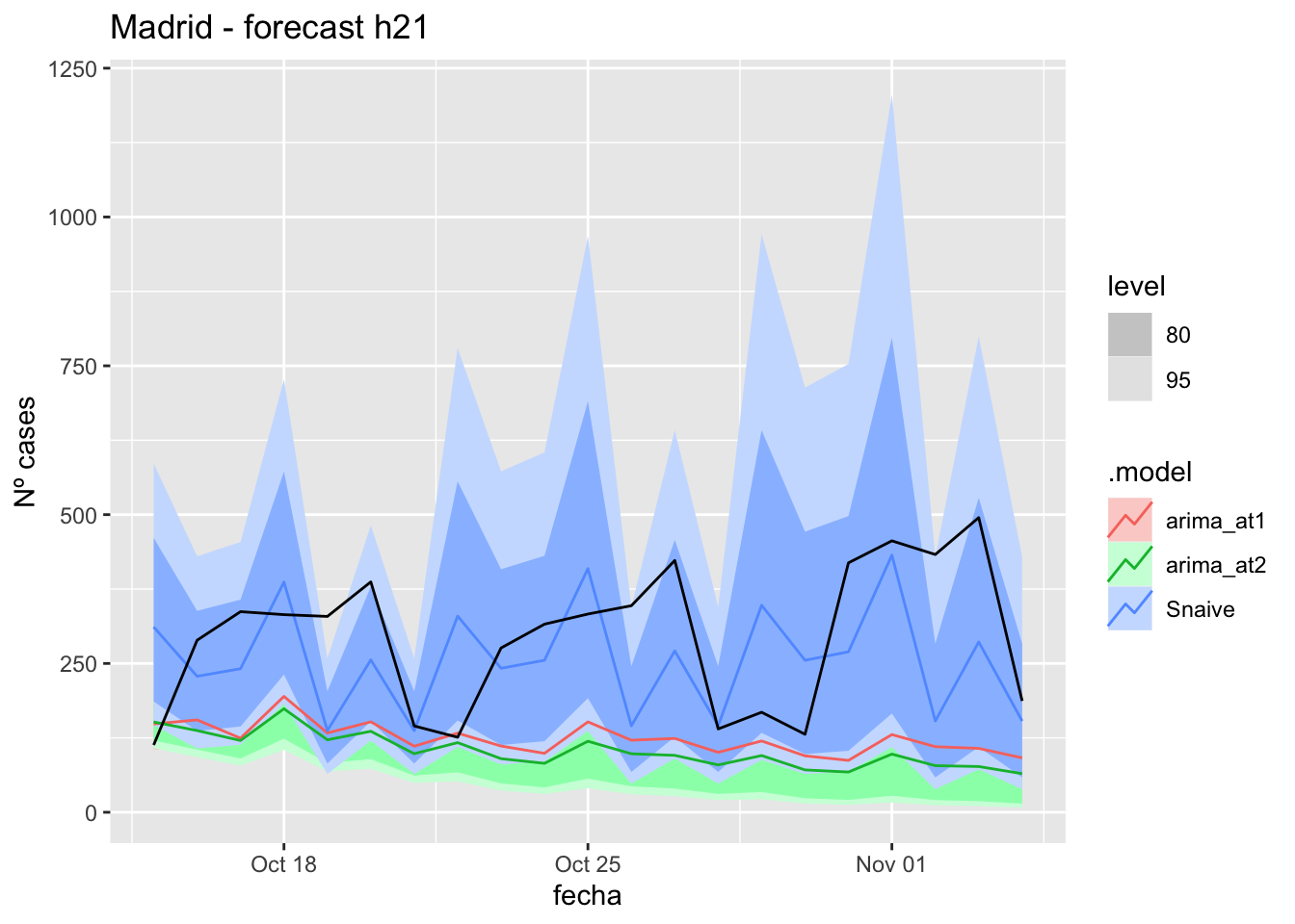
fc_h21 %>%
      autoplot(
            data_Madrid %>%
                  filter(fecha <= as.Date("2021-10-14", format = "%Y-%m-%d")+days(21) &
                               fecha > as.Date("2021-07-01", format = "%Y-%m-%d"))
      ) +
      labs(y = "Nº cases", title = "Madrid - forecast h21")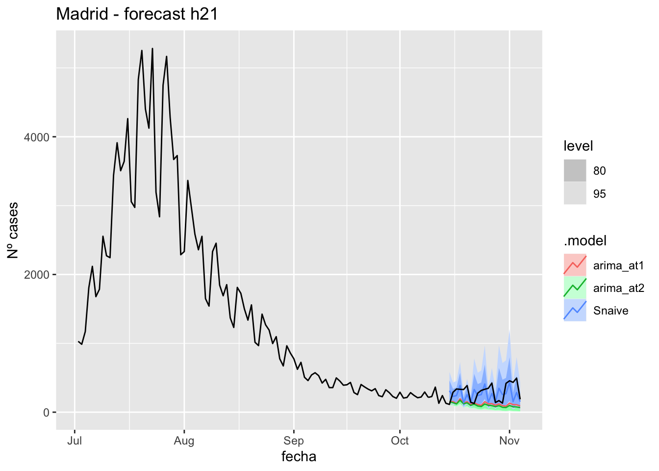
# Accuracy
fabletools::accuracy(fc_h21, data_Madrid)
# A tibble: 3 × 11
.model provincia .type ME RMSE MAE MPE MAPE MASE RMSSE ACF1
<chr> <chr> <chr> <dbl> <dbl> <dbl> <dbl> <dbl> <dbl> <dbl> <dbl>
1 arima_at1 Madrid Test 171. 208. 175. 48.3 51.9 0.411 0.310 0.297
2 arima_at2 Madrid Test 191. 228. 195. 56.1 59.4 0.459 0.339 0.322
3 Snaive Madrid Test 37.6 141. 118. -6.83 48.6 0.278 0.210 0.13190 days
# Plots
fc_h90 %>%
      autoplot(
            data_Madrid_test %>%
                  filter(fecha <= as.Date("2021-10-14", format = "%Y-%m-%d")+days(90))
      ) +
      labs(y = "Nº cases", title = "Madrid - forecast h90")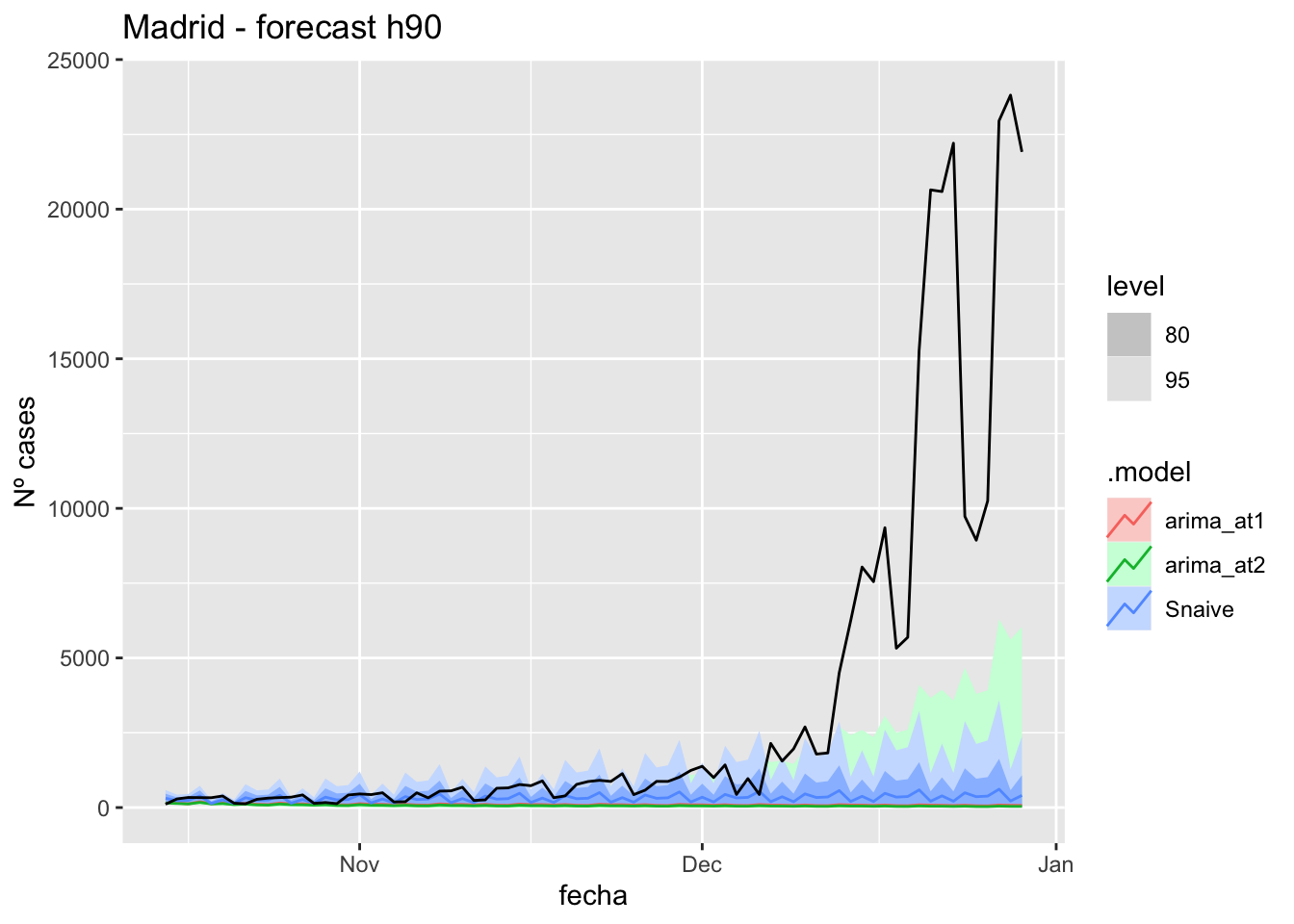
fc_h90 %>%
      autoplot(
            data_Madrid %>%
                  filter(fecha <= as.Date("2021-10-14", format = "%Y-%m-%d")+days(90) &
                               fecha > as.Date("2021-07-01", format = "%Y-%m-%d"))
      ) +
      labs(y = "Nº cases", title = "Madrid - forecast h90")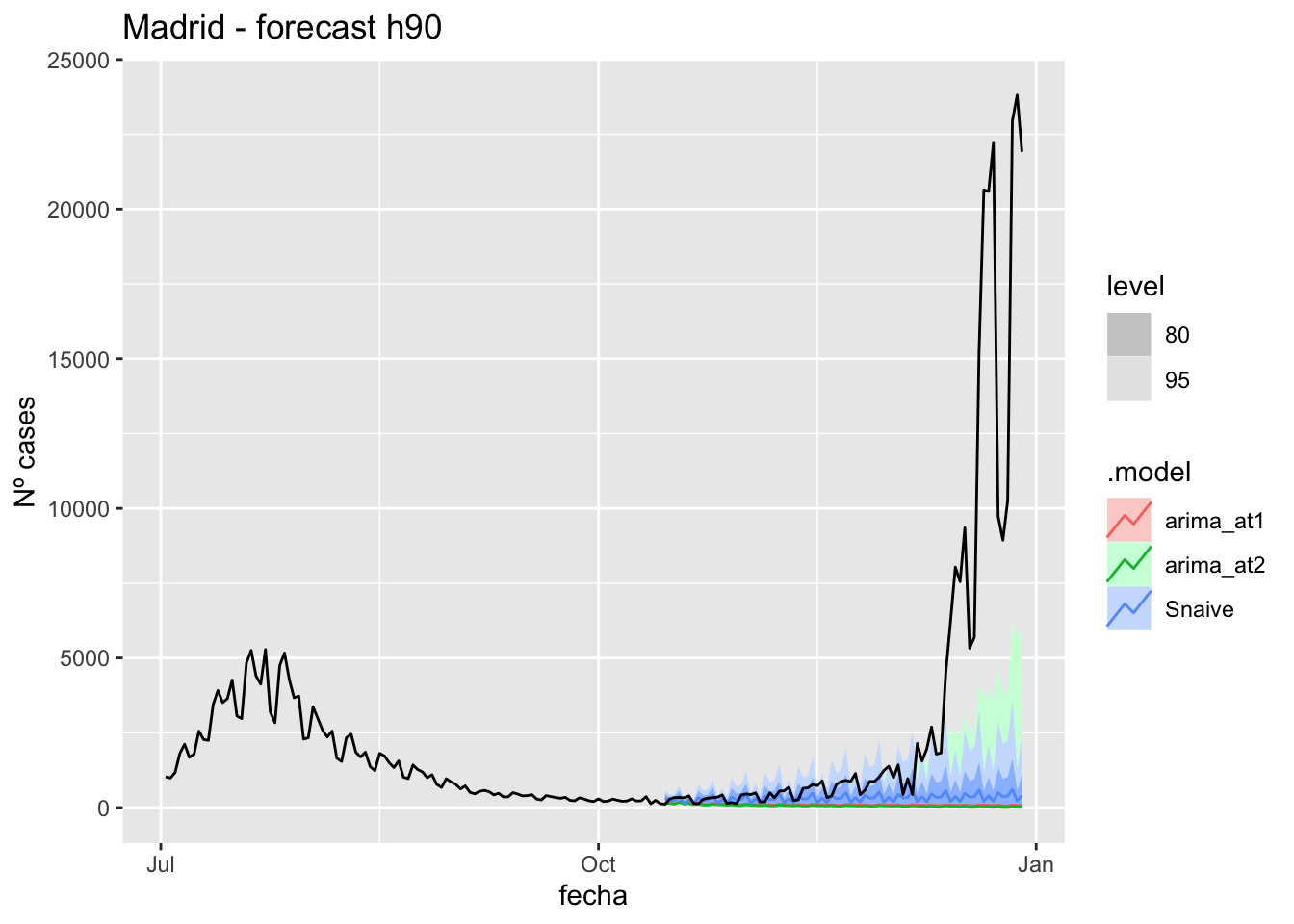
# Accuracy
fabletools::accuracy(fc_h90, data_Madrid)
# A tibble: 3 × 11
.model provincia .type ME RMSE MAE MPE MAPE MASE RMSSE ACF1
<chr> <chr> <chr> <dbl> <dbl> <dbl> <dbl> <dbl> <dbl> <dbl> <dbl>
1 arima_at1 Madrid Test 3379. 7039. 3380. 78.1 79.1 7.96 10.5 0.855
2 arima_at2 Madrid Test 3407. 7055. 3408. 82.8 83.7 8.03 10.5 0.855
3 Snaive Madrid Test 3160. 6905. 3193. 44.5 64.2 7.52 10.3 0.853Malaga
data_Malaga <- covid_data %>%
      filter(provincia == "Málaga") %>%
      filter(fecha > as.Date("2020-06-14", format = "%Y-%m-%d")) %>%
      select(provincia, fecha, num_casos, tmed, mob_flujo) %>%
      drop_na() %>%
      as_tsibble(key = provincia, index = fecha)
data_Malaga
# A tsibble: 563 x 5 [1D]
# Key: provincia [1]
provincia fecha num_casos tmed mob_flujo
<chr> <date> <dbl> <dbl> <dbl>
1 Málaga 2020-06-15 1 27.2 18.9
2 Málaga 2020-06-16 1 27.8 19.8
3 Málaga 2020-06-17 2 26.9 19.9
4 Málaga 2020-06-18 2 21.6 20.0
5 Málaga 2020-06-19 1 24.7 20.1
6 Málaga 2020-06-20 4 22.6 18.1
7 Málaga 2020-06-21 4 22.7 18.8
8 Málaga 2020-06-22 6 25 19.5
9 Málaga 2020-06-23 8 25.6 20.2
10 Málaga 2020-06-24 65 24.5 21.0
# … with 553 more rowsdata_Malaga_train <- data_Malaga %>%
filter(fecha <= as.Date("2021-10-14", format = "%Y-%m-%d"))
summary(data_Malaga_train$fecha) Min. 1st Qu. Median Mean 3rd Qu. Max.
"2020-06-15" "2020-10-14" "2021-02-13" "2021-02-13" "2021-06-14" "2021-10-14" data_Malaga_test <- data_Malaga %>%
filter(fecha > as.Date("2021-10-14", format = "%Y-%m-%d"))
summary(data_Malaga_test$fecha) Min. 1st Qu. Median Mean 3rd Qu. Max.
"2021-10-15" "2021-11-02" "2021-11-21" "2021-11-21" "2021-12-10" "2021-12-29" # Lamba for num_casos
lambda_Malaga_casos <- data_Malaga %>%
features(num_casos, features = guerrero) %>%
pull(lambda_guerrero)
lambda_Malaga_casos[1] 0.2360418# Lamba for average temp
lambda_Malaga_tmed <- data_Malaga %>%
features(tmed, features = guerrero) %>%
pull(lambda_guerrero)
lambda_Malaga_tmed[1] 0.6474133# Lamba for mobility
lambda_Malaga_mobil <- data_Malaga %>%
features(mob_flujo, features = guerrero) %>%
pull(lambda_guerrero)
lambda_Malaga_mobil[1] 1.999927fit_model <- data_Malaga_train %>%
model(
arima_at1 = ARIMA(box_cox(num_casos, lambda_Malaga_casos) ~
box_cox(tmed, lambda_Malaga_tmed) +
box_cox(mob_flujo, lambda_Malaga_mobil)),
arima_at2 = ARIMA(box_cox(num_casos, lambda_Malaga_casos) ~
box_cox(tmed, lambda_Malaga_tmed) +
box_cox(mob_flujo, lambda_Malaga_mobil),
stepwise = FALSE, approx = FALSE),
Snaive = SNAIVE(box_cox(num_casos, lambda_Malaga_casos))
)
# Show and report model
fit_model# A mable: 1 x 4
# Key: provincia [1]
provincia arima_at1
<chr> <model>
1 Málaga <LM w/ ARIMA(4,1,0)(2,1,0)[7] errors>
# … with 2 more variables: arima_at2 <model>, Snaive <model>glance(fit_model)# A tibble: 3 × 9
provincia .model sigma2 log_lik AIC AICc BIC ar_roots ma_roots
<chr> <chr> <dbl> <dbl> <dbl> <dbl> <dbl> <list> <list>
1 Málaga arima_at1 0.610 -559. 1135. 1136. 1173. <cpl [18]> <cpl [0]>
2 Málaga arima_at2 0.524 -526. 1070. 1071. 1108. <cpl [8]> <cpl [10]>
3 Málaga Snaive 2.27 NA NA NA NA <NULL> <NULL> fit_model %>%
pivot_longer(-provincia,
names_to = ".model",
values_to = "orders") %>%
left_join(glance(fit_model), by = c("provincia", ".model")) %>%
arrange(AICc) %>%
select(.model:BIC)# A mable: 3 x 7
# Key: .model [3]
.model orders sigma2 log_lik AIC AICc BIC
<chr> <model> <dbl> <dbl> <dbl> <dbl> <dbl>
1 arima_… <LM w/ ARIMA(1,1,3)(1,1,1)[7] errors> 0.524 -526. 1070. 1071. 1108.
2 arima_… <LM w/ ARIMA(4,1,0)(2,1,0)[7] errors> 0.610 -559. 1135. 1136. 1173.
3 Snaive <SNAIVE> 2.27 NA NA NA NA # We use a Ljung-Box test >> large p-value, confirms residuals are similar / considered to white noise
fit_model %>%
select(Snaive) %>%
gg_tsresiduals()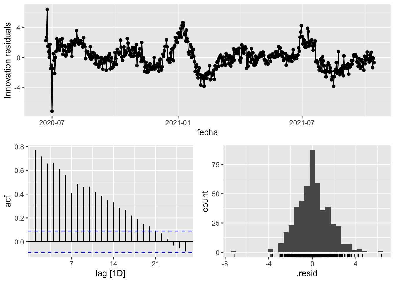
fit_model %>%
      select(arima_at1) %>%
      gg_tsresiduals()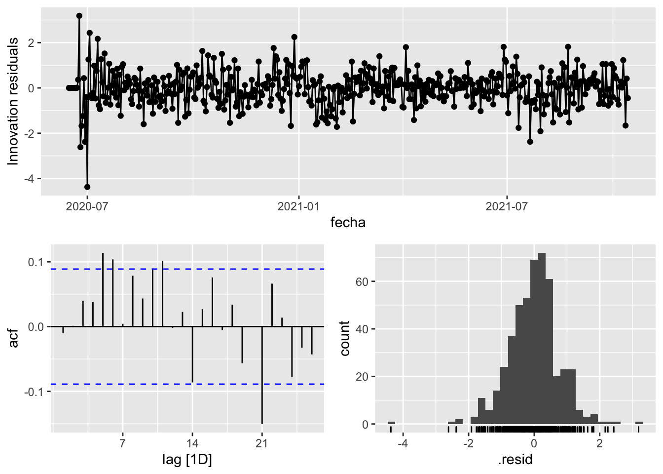
fit_model %>%
      select(arima_at2) %>%
      gg_tsresiduals()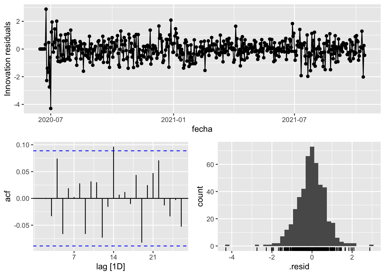
augment(fit_model) %>%
      features(.innov, ljung_box, lag=7)
# A tibble: 3 × 4
provincia .model lb_stat lb_pvalue
<chr> <chr> <dbl> <dbl>
1 Málaga arima_at1 13.3 0.0651
2 Málaga arima_at2 5.64 0.582
3 Málaga Snaive 1373. 0 augment(fit_model) %>%
features(.innov, ljung_box, lag=14)# A tibble: 3 × 4
provincia .model lb_stat lb_pvalue
<chr> <chr> <dbl> <dbl>
1 Málaga arima_at1 30.5 0.00652
2 Málaga arima_at2 16.7 0.273
3 Málaga Snaive 1974. 0 augment(fit_model) %>%
features(.innov, ljung_box, lag=21)# A tibble: 3 × 4
provincia .model lb_stat lb_pvalue
<chr> <chr> <dbl> <dbl>
1 Málaga arima_at1 47.5 0.000795
2 Málaga arima_at2 22.8 0.357
3 Málaga Snaive 2116. 0 augment(fit_model) %>%
features(.innov, ljung_box, lag=90)# A tibble: 3 × 4
provincia .model lb_stat lb_pvalue
<chr> <chr> <dbl> <dbl>
1 Málaga arima_at1 171. 0.000000610
2 Málaga arima_at2 81.4 0.731
3 Málaga Snaive 3229. 0 # To predict future values of infections, we need to pass the model future/prediction values of the complementary variables tmed and mobility
# We are going to select those from the test dataset
data_fc_h7 <- data_Malaga_test %>%
select(-num_casos) %>%
slice(1:7)
data_fc_h14 <- data_Malaga_test %>%
select(-num_casos) %>%
slice(1:14)
data_fc_h21 <- data_Malaga_test %>%
select(-num_casos) %>%
slice(1:21)
data_fc_h90 <- data_Malaga_test %>%
select(-num_casos) %>%
slice(1:90)# Significant spikes out of 30 is still consistent with white noise
# To be sure, use a Ljung-Box test, which has a large p-value, confirming that
# the residuals are similar to white noise.
# Note that the alternative models also passed this test.
#
# Forecast
fc_h7 <- fabletools::forecast(fit_model, new_data = data_fc_h7)
fc_h14 <- fabletools::forecast(fit_model, new_data = data_fc_h14)
fc_h21 <- fabletools::forecast(fit_model, new_data = data_fc_h21)
fc_h90 <- fabletools::forecast(fit_model, new_data = data_fc_h90)7 days
# Plots
fc_h7 %>%
      autoplot(
            data_Malaga_test %>%
                  filter(fecha <= as.Date("2021-10-14", format = "%Y-%m-%d")+days(7))
      ) +
      labs(y = "Nº cases", title = "Malaga - forecast h7")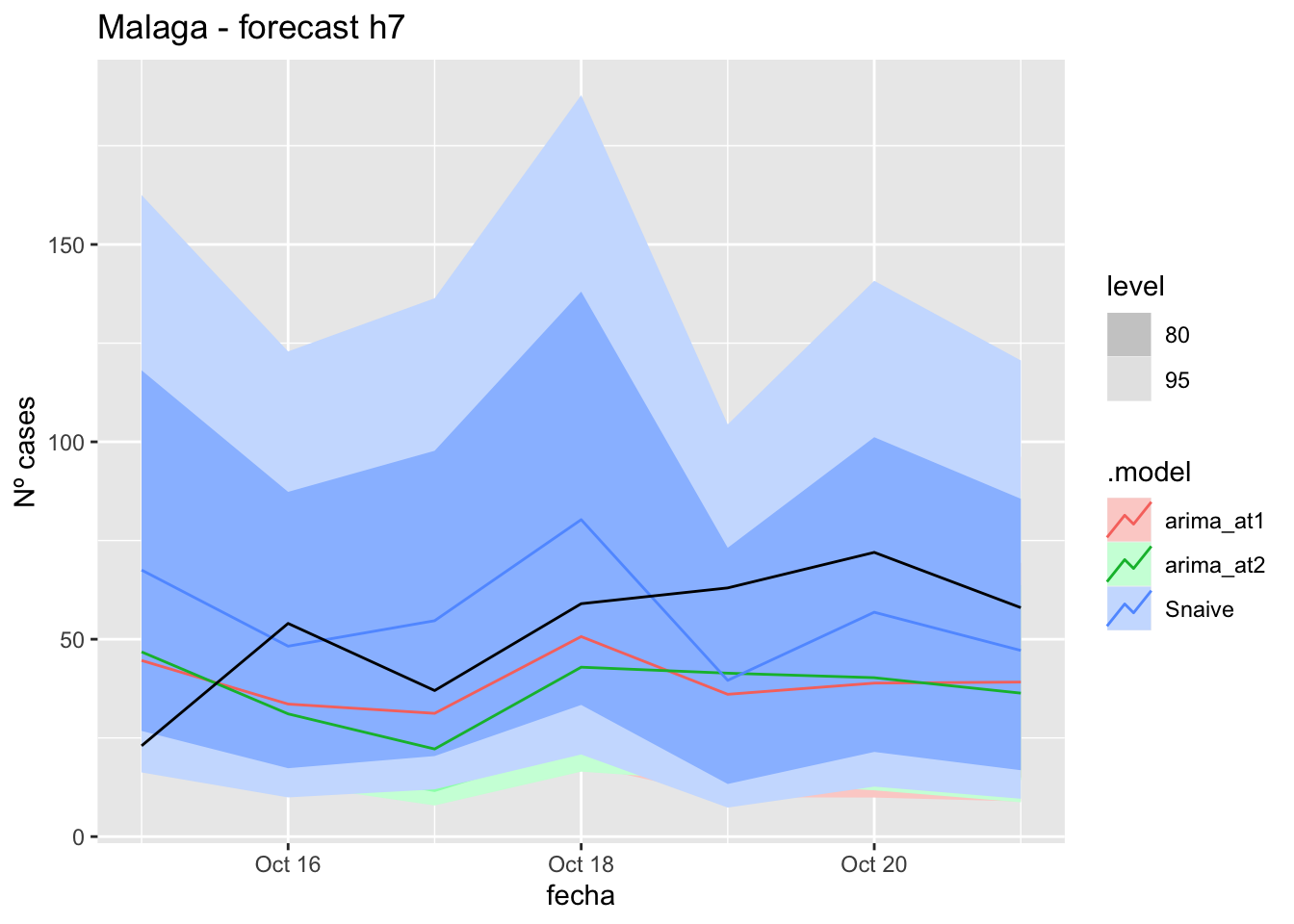
fc_h7 %>%
      autoplot(
            data_Malaga %>%
                  filter(fecha <= as.Date("2021-10-14", format = "%Y-%m-%d")+days(7) &
                               fecha > as.Date("2021-07-01", format = "%Y-%m-%d"))
      ) +
      labs(y = "Nº cases", title = "Malaga - forecast h7")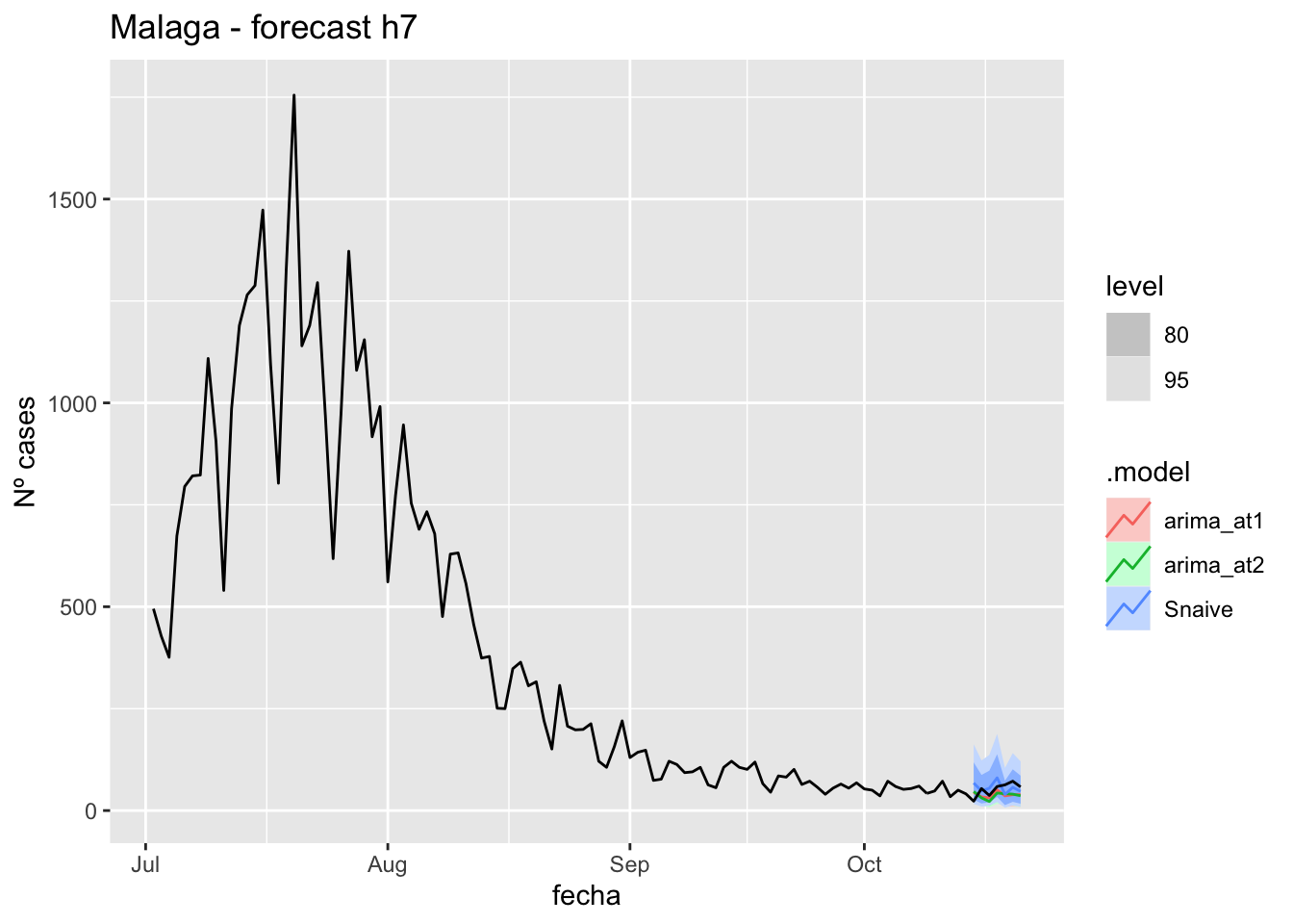
# Accuracy
fabletools::accuracy(fc_h7, data_Malaga)
# A tibble: 3 × 11
.model provincia .type ME RMSE MAE MPE MAPE MASE RMSSE ACF1
<chr> <chr> <chr> <dbl> <dbl> <dbl> <dbl> <dbl> <dbl> <dbl> <dbl>
1 arima_at1 Málaga Test 13.1 21.3 19.3 13.5 40.4 0.196 0.126 0.0270
2 arima_at2 Málaga Test 15.0 22.4 21.8 17.4 47.0 0.221 0.132 -0.0409
3 Snaive Málaga Test -4.05 22.9 19.8 -27.1 52.2 0.201 0.135 0.012414 days
# Plots
fc_h14 %>%
      autoplot(
            data_Malaga_test %>%
                  filter(fecha <= as.Date("2021-10-14", format = "%Y-%m-%d")+days(14))
      ) +
      labs(y = "Nº cases", title = "Malaga - forecast h14")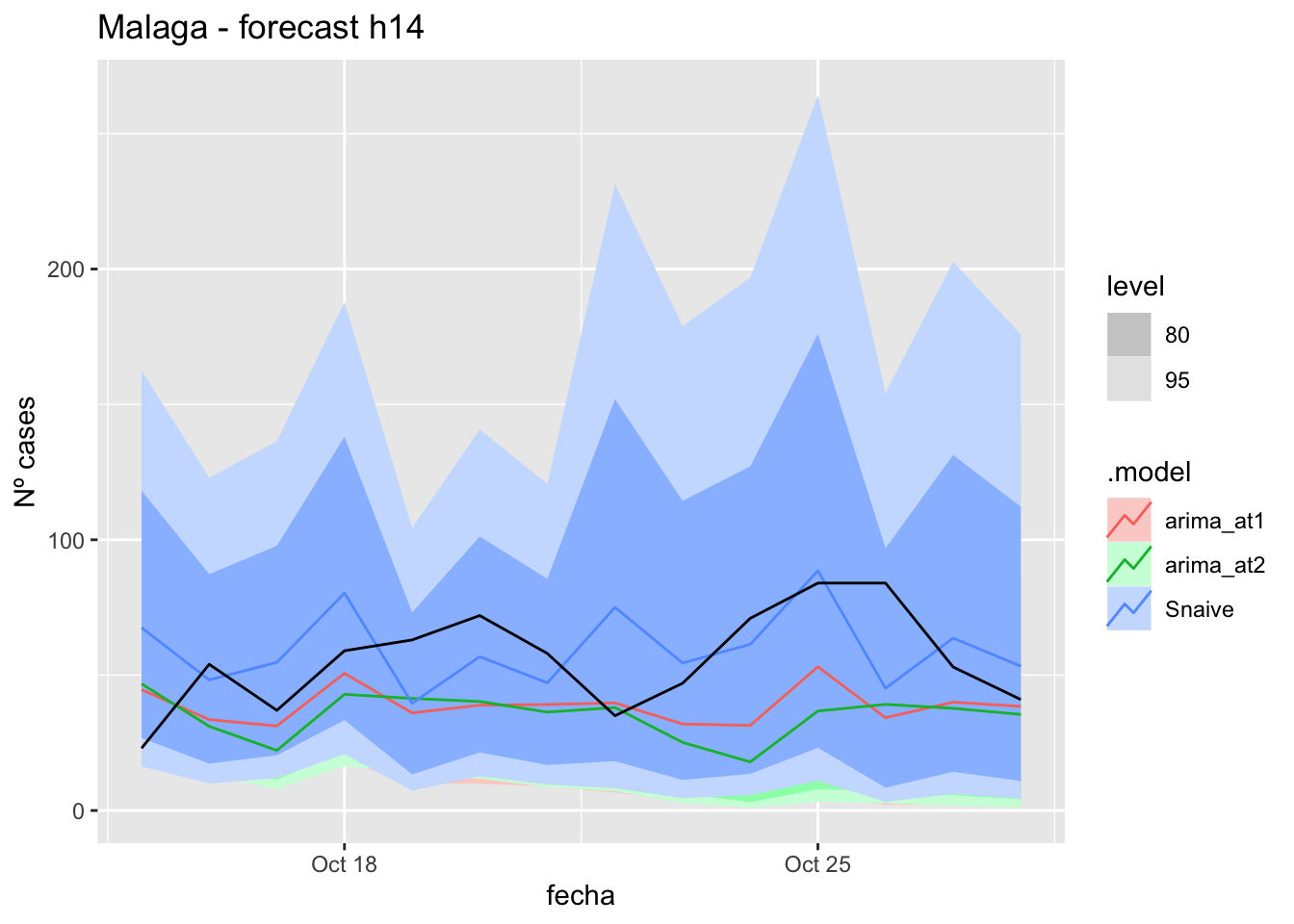
fc_h14 %>%
      autoplot(
            data_Malaga %>%
                  filter(fecha <= as.Date("2021-10-14", format = "%Y-%m-%d")+days(14) &
                               fecha > as.Date("2021-07-01", format = "%Y-%m-%d"))
      ) +
      labs(y = "Nº cases", title = "Malaga - forecast h14")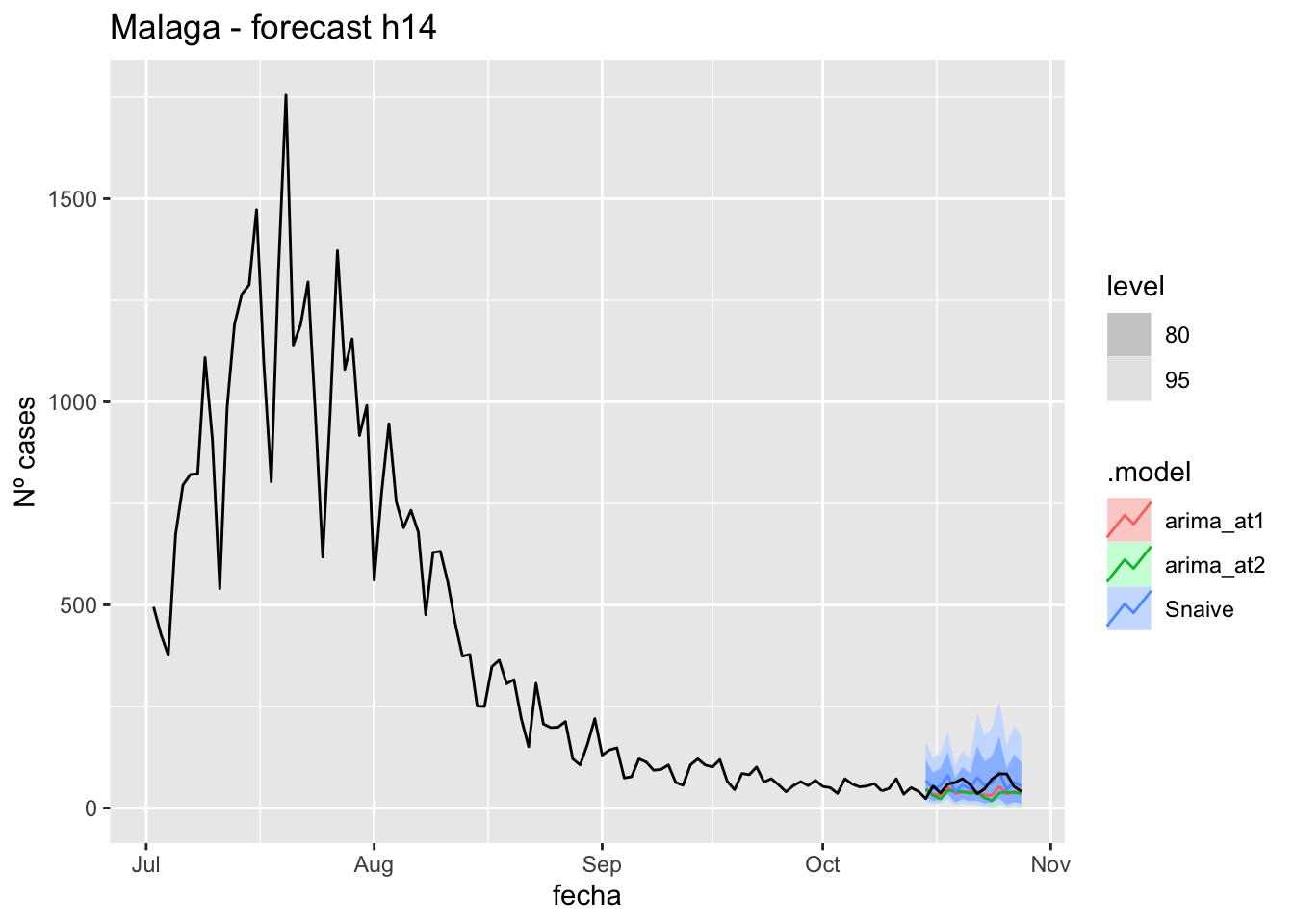
# Accuracy
fabletools::accuracy(fc_h14, data_Malaga)
# A tibble: 3 × 11
.model provincia .type ME RMSE MAE MPE MAPE MASE RMSSE ACF1
<chr> <chr> <chr> <dbl> <dbl> <dbl> <dbl> <dbl> <dbl> <dbl> <dbl>
1 arima_at1 Málaga Test 17.0 24.8 20.8 21.1 36.5 0.211 0.146 0.151
2 arima_at2 Málaga Test 20.7 28.4 24.5 27.6 43.6 0.249 0.168 0.258
3 Snaive Málaga Test -3.93 22.7 18.7 -22.6 43.6 0.190 0.134 -0.097121 days
# Plots
fc_h21 %>%
      autoplot(
            data_Malaga_test %>%
                  filter(fecha <= as.Date("2021-10-14", format = "%Y-%m-%d")+days(21))
      ) +
      labs(y = "Nº cases", title = "Malaga - forecast h21")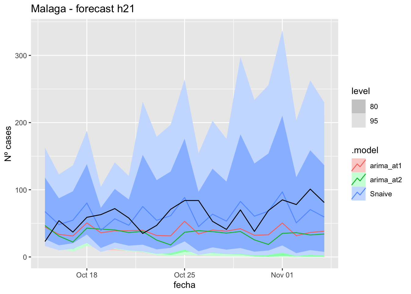
fc_h21 %>%
      autoplot(
            data_Malaga %>%
                  filter(fecha <= as.Date("2021-10-14", format = "%Y-%m-%d")+days(21) &
                               fecha > as.Date("2021-07-01", format = "%Y-%m-%d"))
      ) +
      labs(y = "Nº cases", title = "Malaga - forecast h21")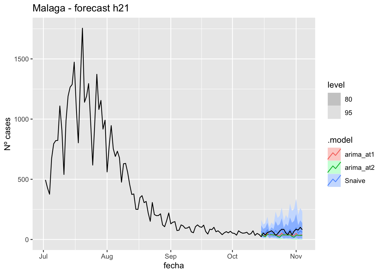
# Accuracy
fabletools::accuracy(fc_h21, data_Malaga)
# A tibble: 3 × 11
.model provincia .type ME RMSE MAE MPE MAPE MASE RMSSE ACF1
<chr> <chr> <chr> <dbl> <dbl> <dbl> <dbl> <dbl> <dbl> <dbl> <dbl>
1 arima_at1 Málaga Test 23.6 30.9 26.1 29.5 39.7 0.265 0.182 0.314
2 arima_at2 Málaga Test 28.2 35.3 30.7 37.0 47.6 0.312 0.208 0.341
3 Snaive Málaga Test -1.04 22.0 18.6 -15.0 37.9 0.188 0.130 0.088690 days
# Plots
fc_h90 %>%
      autoplot(
            data_Malaga_test %>%
                  filter(fecha <= as.Date("2021-10-14", format = "%Y-%m-%d")+days(90))
      ) +
      labs(y = "Nº cases", title = "Malaga - forecast h90")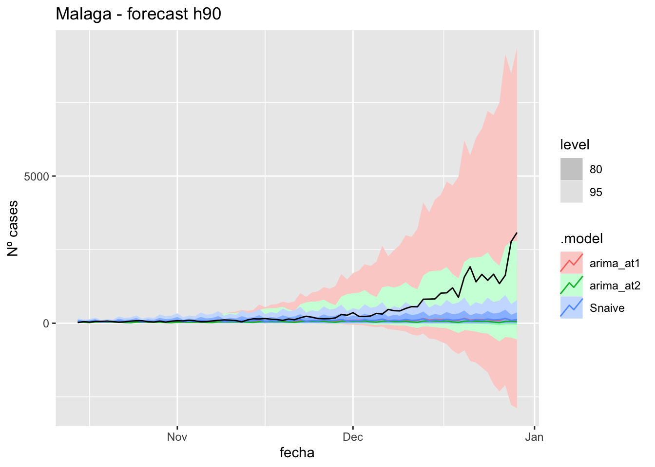
fc_h90 %>%
      autoplot(
            data_Malaga %>%
                  filter(fecha <= as.Date("2021-10-14", format = "%Y-%m-%d")+days(90) &
                               fecha > as.Date("2021-07-01", format = "%Y-%m-%d"))
      ) +
      labs(y = "Nº cases", title = "Malaga - forecast h90")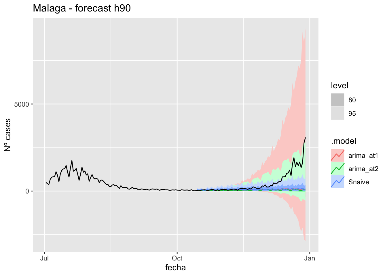
# Accuracy
fabletools::accuracy(fc_h90, data_Malaga)
# A tibble: 3 × 11
.model provincia .type ME RMSE MAE MPE MAPE MASE RMSSE ACF1
<chr> <chr> <chr> <dbl> <dbl> <dbl> <dbl> <dbl> <dbl> <dbl> <dbl>
1 arima_at1 Málaga Test 380. 720. 382. 55.6 59.2 3.87 4.25 0.826
2 arima_at2 Málaga Test 408. 749. 409. 65.2 68.5 4.16 4.42 0.835
3 Snaive Málaga Test 367. 720. 375. 35.8 56.6 3.81 4.25 0.827Sevilla
data_Sevilla <- covid_data %>%
      filter(provincia == "Sevilla") %>%
      filter(fecha > as.Date("2020-06-14", format = "%Y-%m-%d")) %>%
      select(provincia, fecha, num_casos, tmed, mob_flujo) %>%
      drop_na() %>%
      as_tsibble(key = provincia, index = fecha)
data_Sevilla
# A tsibble: 563 x 5 [1D]
# Key: provincia [1]
provincia fecha num_casos tmed mob_flujo
<chr> <date> <dbl> <dbl> <dbl>
1 Sevilla 2020-06-15 2 23.1 19.9
2 Sevilla 2020-06-16 1 24.0 20.8
3 Sevilla 2020-06-17 0 24.9 21.1
4 Sevilla 2020-06-18 0 25.8 21.3
5 Sevilla 2020-06-19 0 26.6 21.2
6 Sevilla 2020-06-20 0 27.5 18.0
7 Sevilla 2020-06-21 0 28.4 18.9
8 Sevilla 2020-06-22 1 29.3 19.8
9 Sevilla 2020-06-23 0 30.2 20.7
10 Sevilla 2020-06-24 1 29.4 21.6
# … with 553 more rowsdata_Sevilla_train <- data_Sevilla %>%
filter(fecha <= as.Date("2021-10-14", format = "%Y-%m-%d"))
summary(data_Sevilla_train$fecha) Min. 1st Qu. Median Mean 3rd Qu. Max.
"2020-06-15" "2020-10-14" "2021-02-13" "2021-02-13" "2021-06-14" "2021-10-14" data_Sevilla_test <- data_Sevilla %>%
filter(fecha > as.Date("2021-10-14", format = "%Y-%m-%d"))
summary(data_Sevilla_test$fecha) Min. 1st Qu. Median Mean 3rd Qu. Max.
"2021-10-15" "2021-11-02" "2021-11-21" "2021-11-21" "2021-12-10" "2021-12-29" # Lamba for num_casos
lambda_Sevilla_casos <- data_Sevilla %>%
features(num_casos, features = guerrero) %>%
pull(lambda_guerrero)
lambda_Sevilla_casos[1] 0.2191951# Lamba for average temp
lambda_Sevilla_tmed <- data_Sevilla %>%
features(tmed, features = guerrero) %>%
pull(lambda_guerrero)
lambda_Sevilla_tmed[1] 1.057197# Lamba for mobility
lambda_Sevilla_mobil <- data_Sevilla %>%
features(mob_flujo, features = guerrero) %>%
pull(lambda_guerrero)
lambda_Sevilla_mobil[1] 0.7413917fit_model <- data_Sevilla_train %>%
model(
arima_at1 = ARIMA(box_cox(num_casos, lambda_Sevilla_casos) ~
box_cox(tmed, lambda_Sevilla_tmed) +
box_cox(mob_flujo, lambda_Sevilla_mobil)),
arima_at2 = ARIMA(box_cox(num_casos, lambda_Sevilla_casos) ~
box_cox(tmed, lambda_Sevilla_tmed) +
box_cox(mob_flujo, lambda_Sevilla_mobil),
stepwise = FALSE, approx = FALSE),
Snaive = SNAIVE(box_cox(num_casos, lambda_Sevilla_casos))
)
# Show and report model
fit_model# A mable: 1 x 4
# Key: provincia [1]
provincia arima_at1
<chr> <model>
1 Sevilla <LM w/ ARIMA(3,1,0)(2,1,0)[7] errors>
# … with 2 more variables: arima_at2 <model>, Snaive <model>glance(fit_model)# A tibble: 3 × 9
provincia .model sigma2 log_lik AIC AICc BIC ar_roots ma_roots
<chr> <chr> <dbl> <dbl> <dbl> <dbl> <dbl> <list> <list>
1 Sevilla arima_at1 0.937 -662. 1341. 1341. 1374. <cpl [17]> <cpl [0]>
2 Sevilla arima_at2 0.854 -643. 1304. 1304. 1342. <cpl [7]> <cpl [11]>
3 Sevilla Snaive 2.33 NA NA NA NA <NULL> <NULL> fit_model %>%
pivot_longer(-provincia,
names_to = ".model",
values_to = "orders") %>%
left_join(glance(fit_model), by = c("provincia", ".model")) %>%
arrange(AICc) %>%
select(.model:BIC)# A mable: 3 x 7
# Key: .model [3]
.model orders sigma2 log_lik AIC AICc BIC
<chr> <model> <dbl> <dbl> <dbl> <dbl> <dbl>
1 arima_… <LM w/ ARIMA(0,1,4)(1,1,1)[7] errors> 0.854 -643. 1304. 1304. 1342.
2 arima_… <LM w/ ARIMA(3,1,0)(2,1,0)[7] errors> 0.937 -662. 1341. 1341. 1374.
3 Snaive <SNAIVE> 2.33 NA NA NA NA # We use a Ljung-Box test >> large p-value, confirms residuals are similar / considered to white noise
fit_model %>%
select(Snaive) %>%
gg_tsresiduals()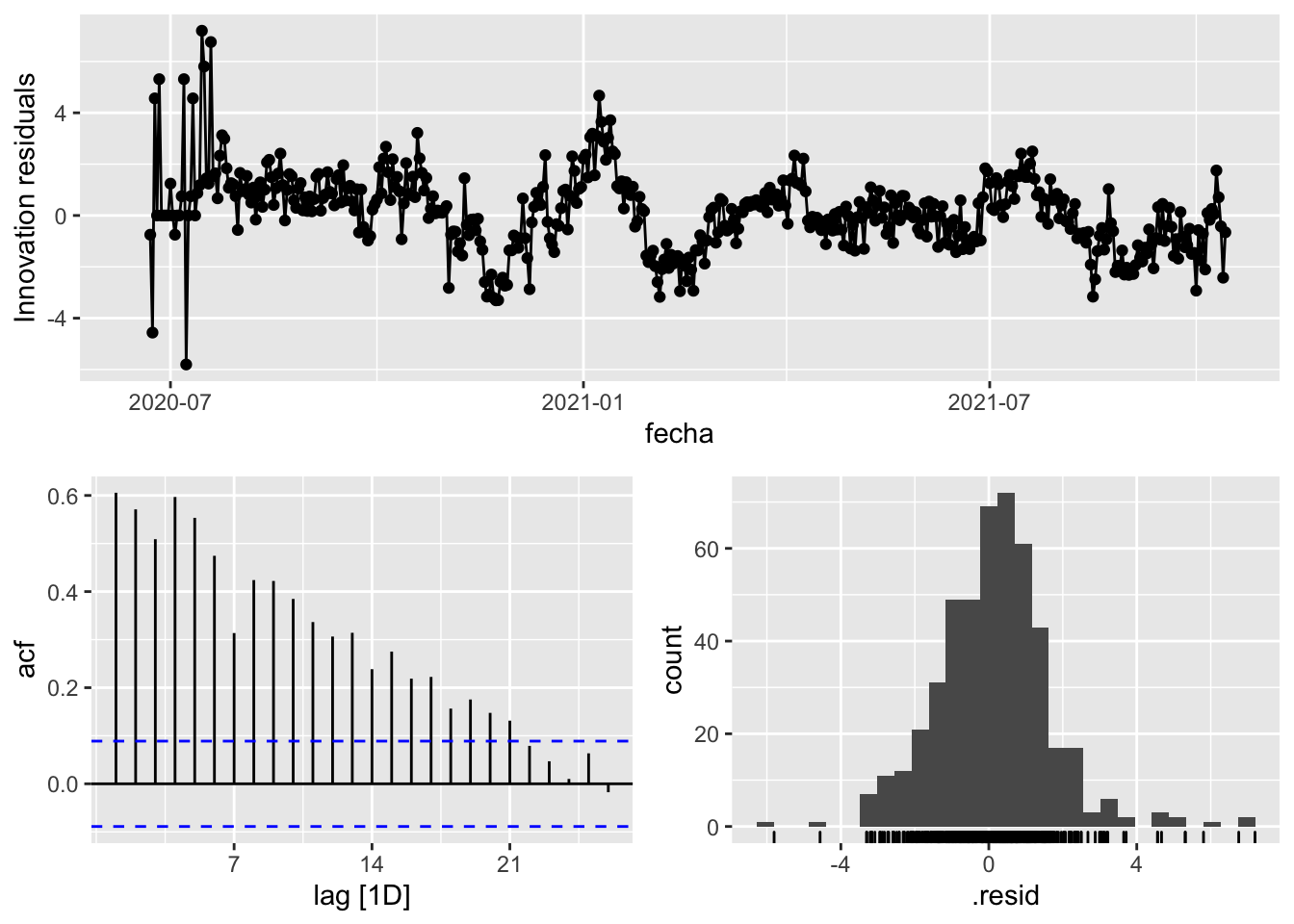
fit_model %>%
      select(arima_at1) %>%
      gg_tsresiduals()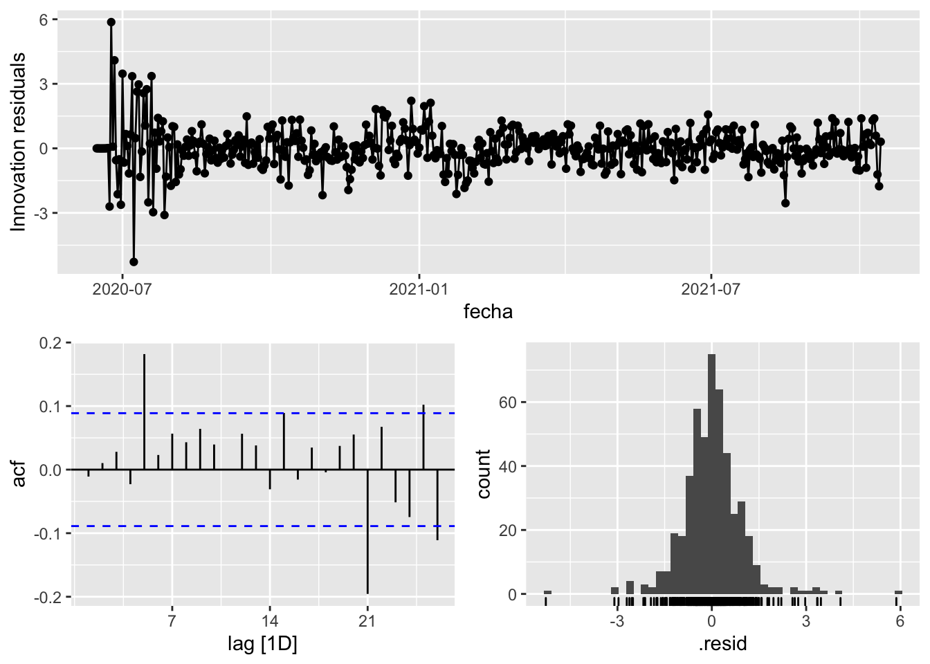
fit_model %>%
      select(arima_at2) %>%
      gg_tsresiduals()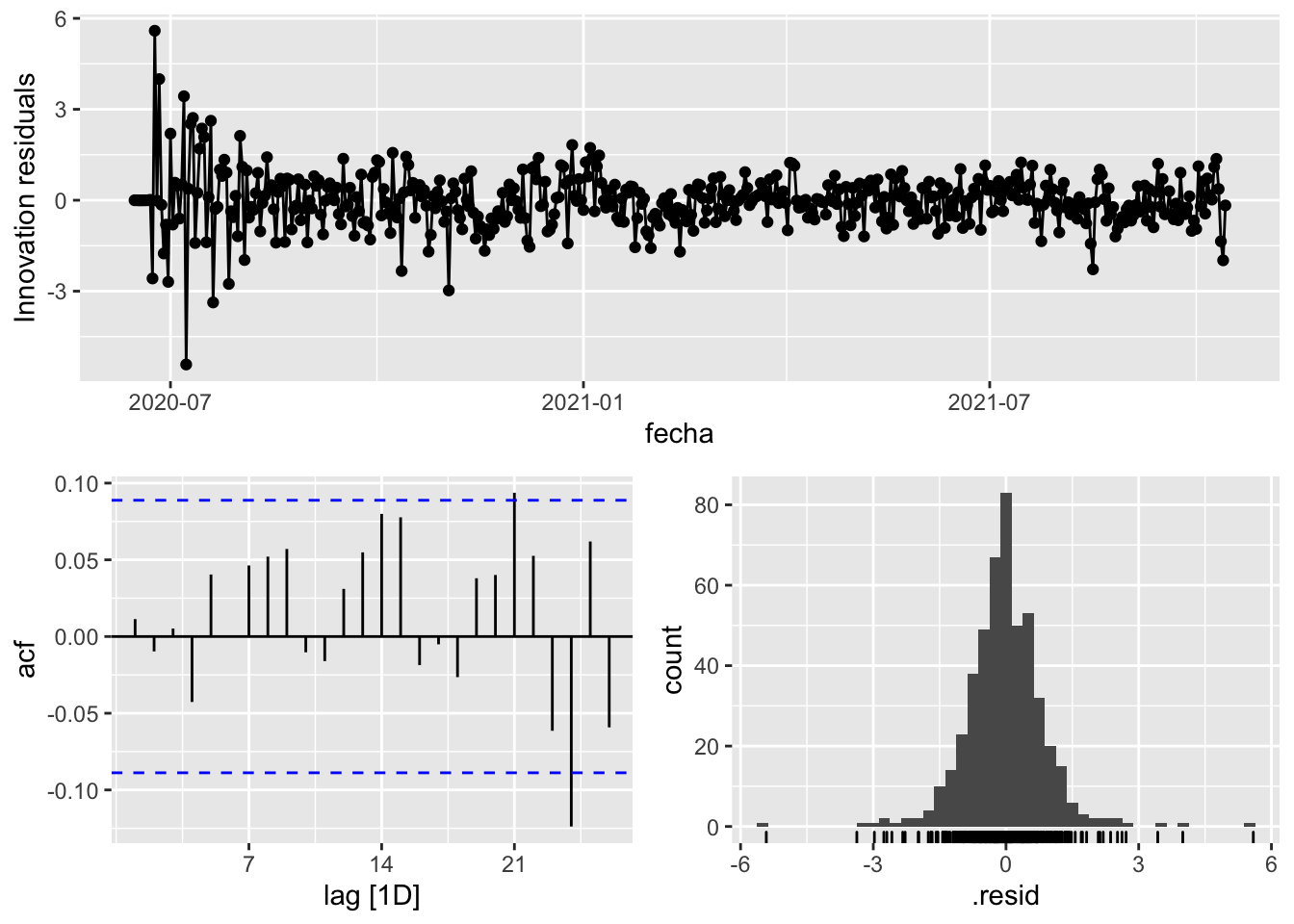
augment(fit_model) %>%
      features(.innov, ljung_box, lag=7)
# A tibble: 3 × 4
provincia .model lb_stat lb_pvalue
<chr> <chr> <dbl> <dbl>
1 Sevilla arima_at1 18.9 0.00840
2 Sevilla arima_at2 2.89 0.895
3 Sevilla Snaive 941. 0 augment(fit_model) %>%
features(.innov, ljung_box, lag=14)# A tibble: 3 × 4
provincia .model lb_stat lb_pvalue
<chr> <chr> <dbl> <dbl>
1 Sevilla arima_at1 25.5 0.0300
2 Sevilla arima_at2 11.3 0.666
3 Sevilla Snaive 1369. 0 augment(fit_model) %>%
features(.innov, ljung_box, lag=21)# A tibble: 3 × 4
provincia .model lb_stat lb_pvalue
<chr> <chr> <dbl> <dbl>
1 Sevilla arima_at1 52.1 0.000188
2 Sevilla arima_at2 20.9 0.466
3 Sevilla Snaive 1503. 0 augment(fit_model) %>%
features(.innov, ljung_box, lag=90)# A tibble: 3 × 4
provincia .model lb_stat lb_pvalue
<chr> <chr> <dbl> <dbl>
1 Sevilla arima_at1 163. 0.00000369
2 Sevilla arima_at2 106. 0.120
3 Sevilla Snaive 2164. 0 # To predict future values of infections, we need to pass the model future/prediction values of the complementary variables tmed and mobility
# We are going to select those from the test dataset
data_fc_h7 <- data_Sevilla_test %>%
select(-num_casos) %>%
slice(1:7)
data_fc_h14 <- data_Sevilla_test %>%
select(-num_casos) %>%
slice(1:14)
data_fc_h21 <- data_Sevilla_test %>%
select(-num_casos) %>%
slice(1:21)
data_fc_h90 <- data_Sevilla_test %>%
select(-num_casos) %>%
slice(1:90)# Significant spikes out of 30 is still consistent with white noise
# To be sure, use a Ljung-Box test, which has a large p-value, confirming that
# the residuals are similar to white noise.
# Note that the alternative models also passed this test.
#
# Forecast
fc_h7 <- fabletools::forecast(fit_model, new_data = data_fc_h7)
fc_h14 <- fabletools::forecast(fit_model, new_data = data_fc_h14)
fc_h21 <- fabletools::forecast(fit_model, new_data = data_fc_h21)
fc_h90 <- fabletools::forecast(fit_model, new_data = data_fc_h90)7 days
# Plots
fc_h7 %>%
autoplot(
data_Sevilla_test %>%
filter(fecha <= as.Date("2021-10-14", format = "%Y-%m-%d")+days(7))
) +
labs(y = "Nº cases", title = "Sevilla - forecast h7")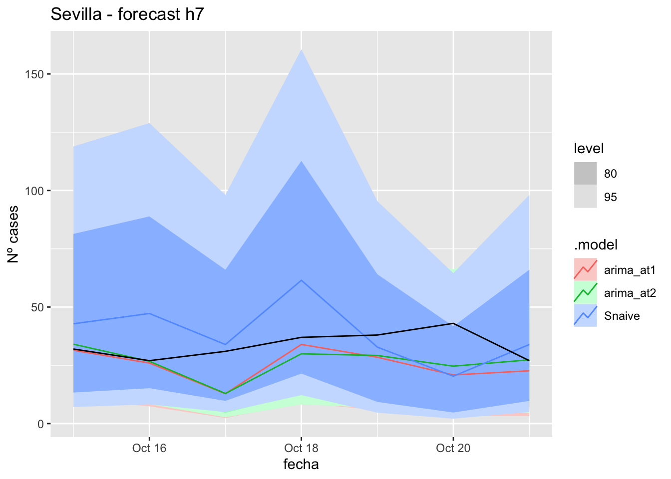
fc_h7 %>%
autoplot(
data_Sevilla %>%
filter(fecha <= as.Date("2021-10-14", format = "%Y-%m-%d")+days(7) &
fecha > as.Date("2021-07-01", format = "%Y-%m-%d"))
) +
labs(y = "Nº cases", title = "Sevilla - forecast h7")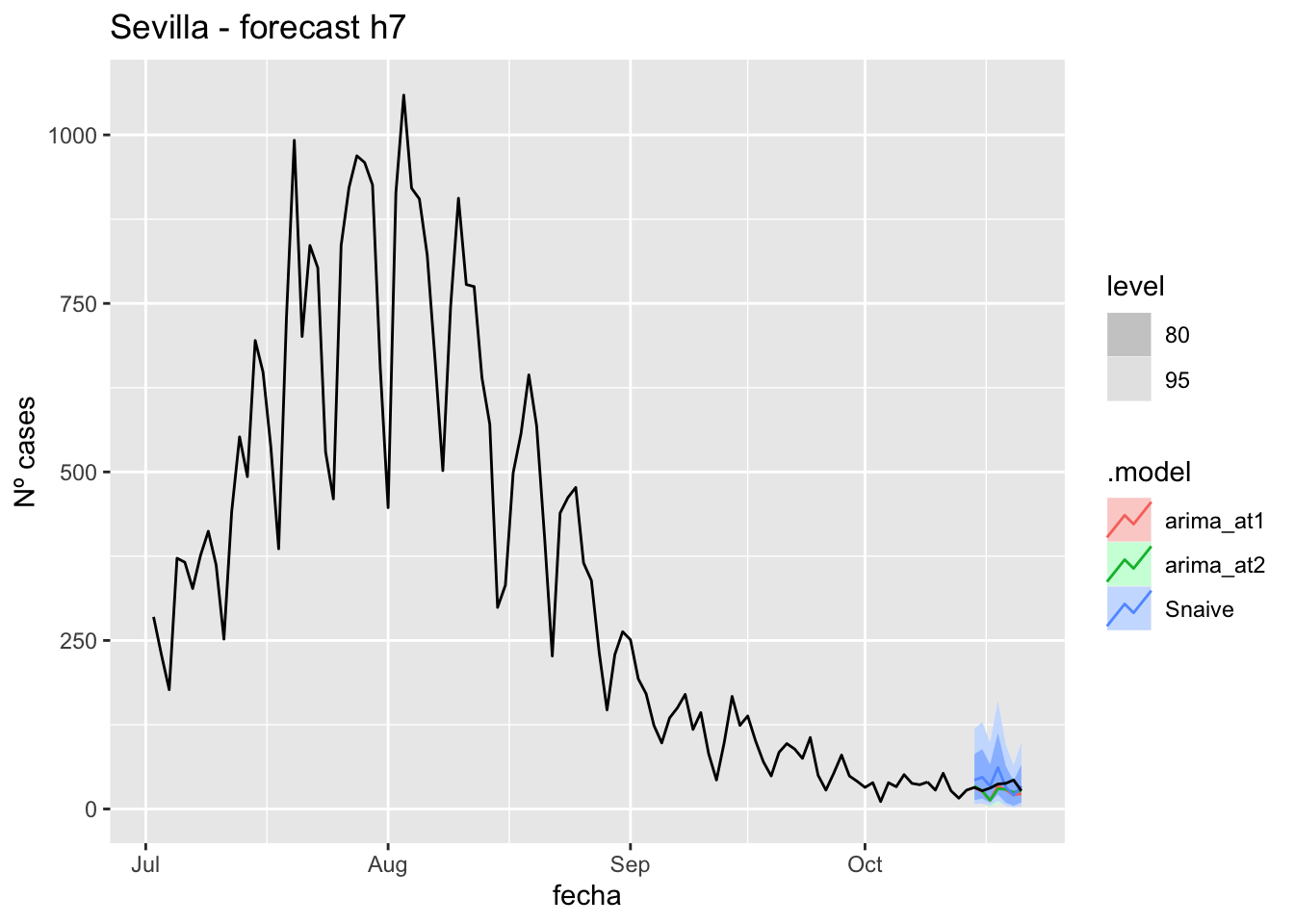
# Accuracy
fabletools::accuracy(fc_h7, data_Sevilla)# A tibble: 3 × 11
.model provincia .type ME RMSE MAE MPE MAPE MASE RMSSE ACF1
<chr> <chr> <chr> <dbl> <dbl> <dbl> <dbl> <dbl> <dbl> <dbl> <dbl>
1 arima_at1 Sevilla Test 8.40 11.6 8.40 23.6 23.6 0.0830 0.0735 -0.252
2 arima_at2 Sevilla Test 7.16 10.7 7.85 19.5 21.7 0.0776 0.0676 -0.181
3 Snaive Sevilla Test -5.36 15.7 13.3 -20.5 39.5 0.132 0.0995 0.032014 days
# Plots
fc_h14 %>%
autoplot(
data_Sevilla_test %>%
filter(fecha <= as.Date("2021-10-14", format = "%Y-%m-%d")+days(14))
) +
labs(y = "Nº cases", title = "Sevilla - forecast h14")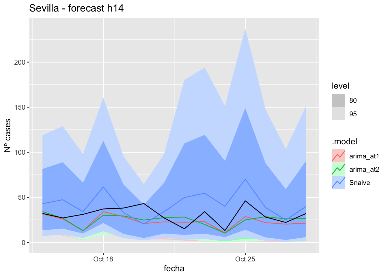
fc_h14 %>%
autoplot(
data_Sevilla %>%
filter(fecha <= as.Date("2021-10-14", format = "%Y-%m-%d")+days(14) &
fecha > as.Date("2021-07-01", format = "%Y-%m-%d"))
) +
labs(y = "Nº cases", title = "Sevilla - forecast h14")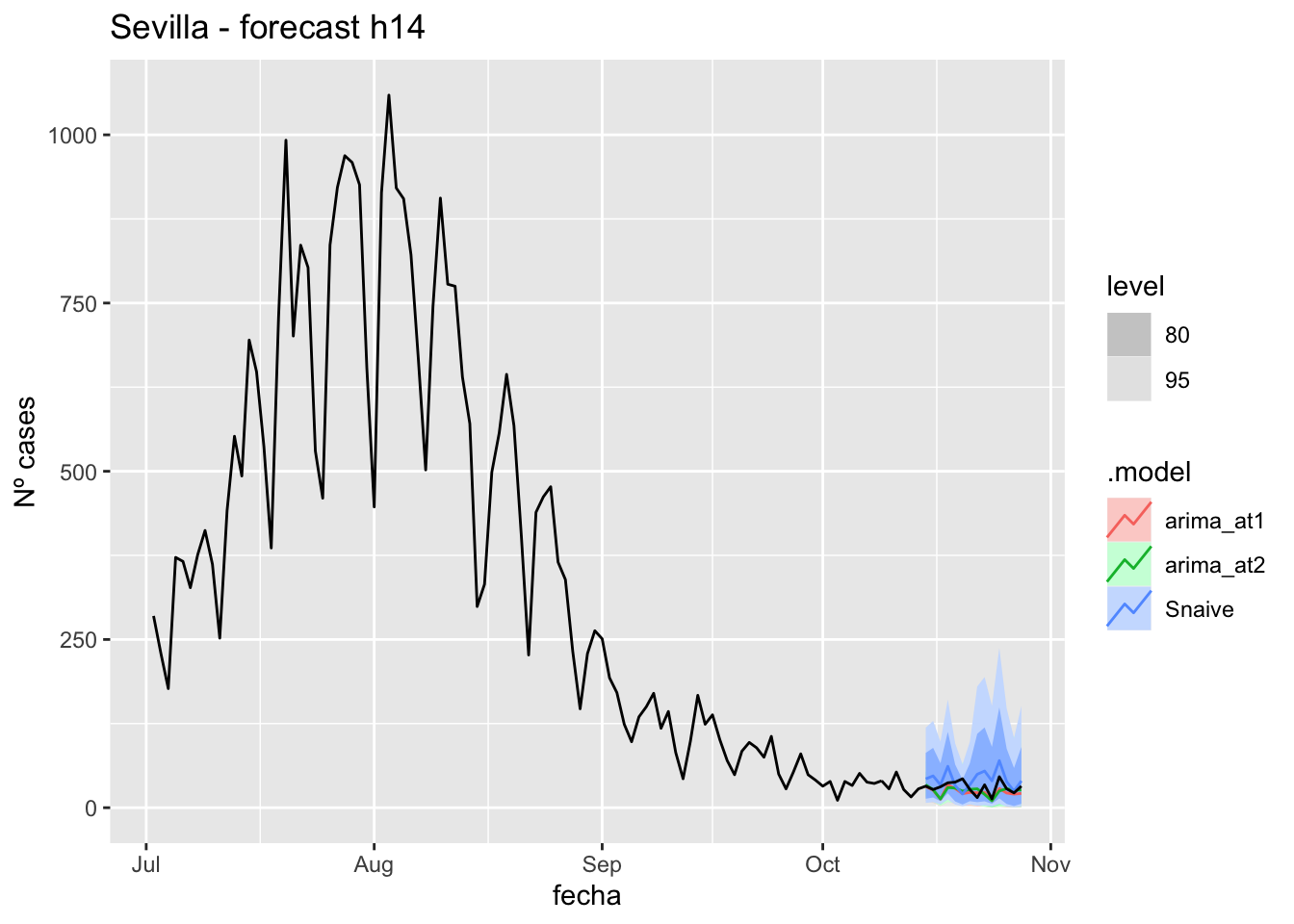
# Accuracy
fabletools::accuracy(fc_h14, data_Sevilla)# A tibble: 3 × 11
.model provincia .type ME RMSE MAE MPE MAPE MASE RMSSE ACF1
<chr> <chr> <chr> <dbl> <dbl> <dbl> <dbl> <dbl> <dbl> <dbl> <dbl>
1 arima_at1 Sevilla Test 7.24 10.6 8.27 19.3 26.2 0.0817 0.0674 -0.229
2 arima_at2 Sevilla Test 5.47 10.9 8.30 11.2 27.5 0.0820 0.0693 -0.153
3 Snaive Sevilla Test -11.8 18.6 15.7 -54.9 64.3 0.155 0.118 0.26921 days
# Plots
fc_h21 %>%
autoplot(
data_Sevilla_test %>%
filter(fecha <= as.Date("2021-10-14", format = "%Y-%m-%d")+days(21))
) +
labs(y = "Nº cases", title = "Sevilla - forecast h21")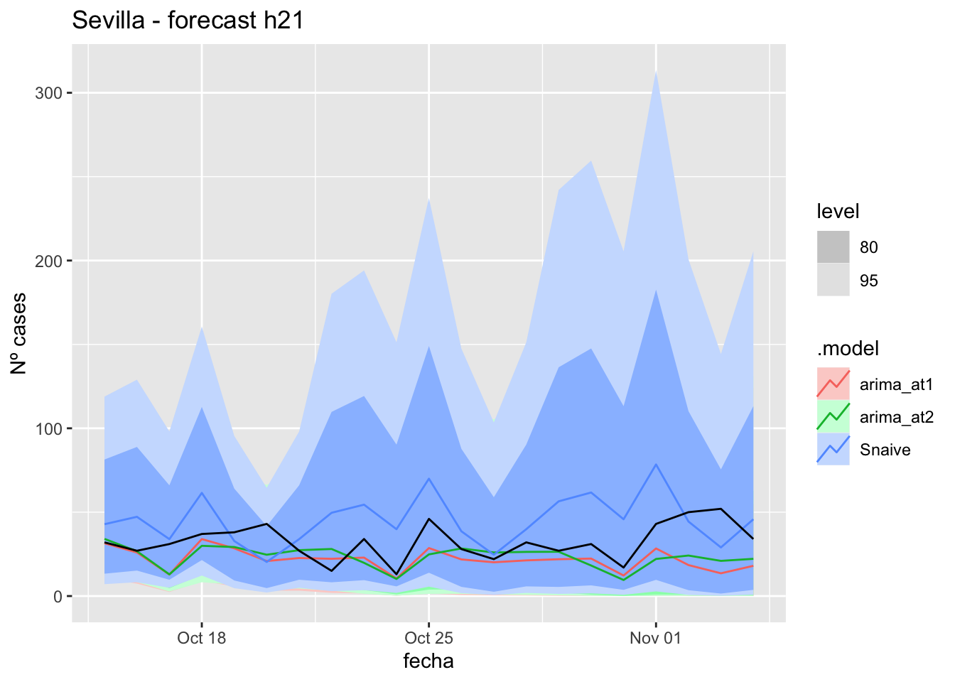
fc_h21 %>%
autoplot(
data_Sevilla %>%
filter(fecha <= as.Date("2021-10-14", format = "%Y-%m-%d")+days(21) &
fecha > as.Date("2021-07-01", format = "%Y-%m-%d"))
) +
labs(y = "Nº cases", title = "Sevilla - forecast h21")
# Accuracy
fabletools::accuracy(fc_h21, data_Sevilla)# A tibble: 3 × 11
.model provincia .type ME RMSE MAE MPE MAPE MASE RMSSE ACF1
<chr> <chr> <chr> <dbl> <dbl> <dbl> <dbl> <dbl> <dbl> <dbl> <dbl>
1 arima_at1 Sevilla Test 10.5 14.9 11.2 26.8 31.4 0.110 0.0943 0.324
2 arima_at2 Sevilla Test 8.90 14.0 10.8 20.9 31.8 0.107 0.0886 0.226
3 Snaive Sevilla Test -13.0 21.2 18.3 -57.5 69.1 0.181 0.134 0.32790 days
# Plots
fc_h90 %>%
autoplot(
data_Sevilla_test %>%
filter(fecha <= as.Date("2021-10-14", format = "%Y-%m-%d")+days(90))
) +
labs(y = "Nº cases", title = "Sevilla - forecast h90")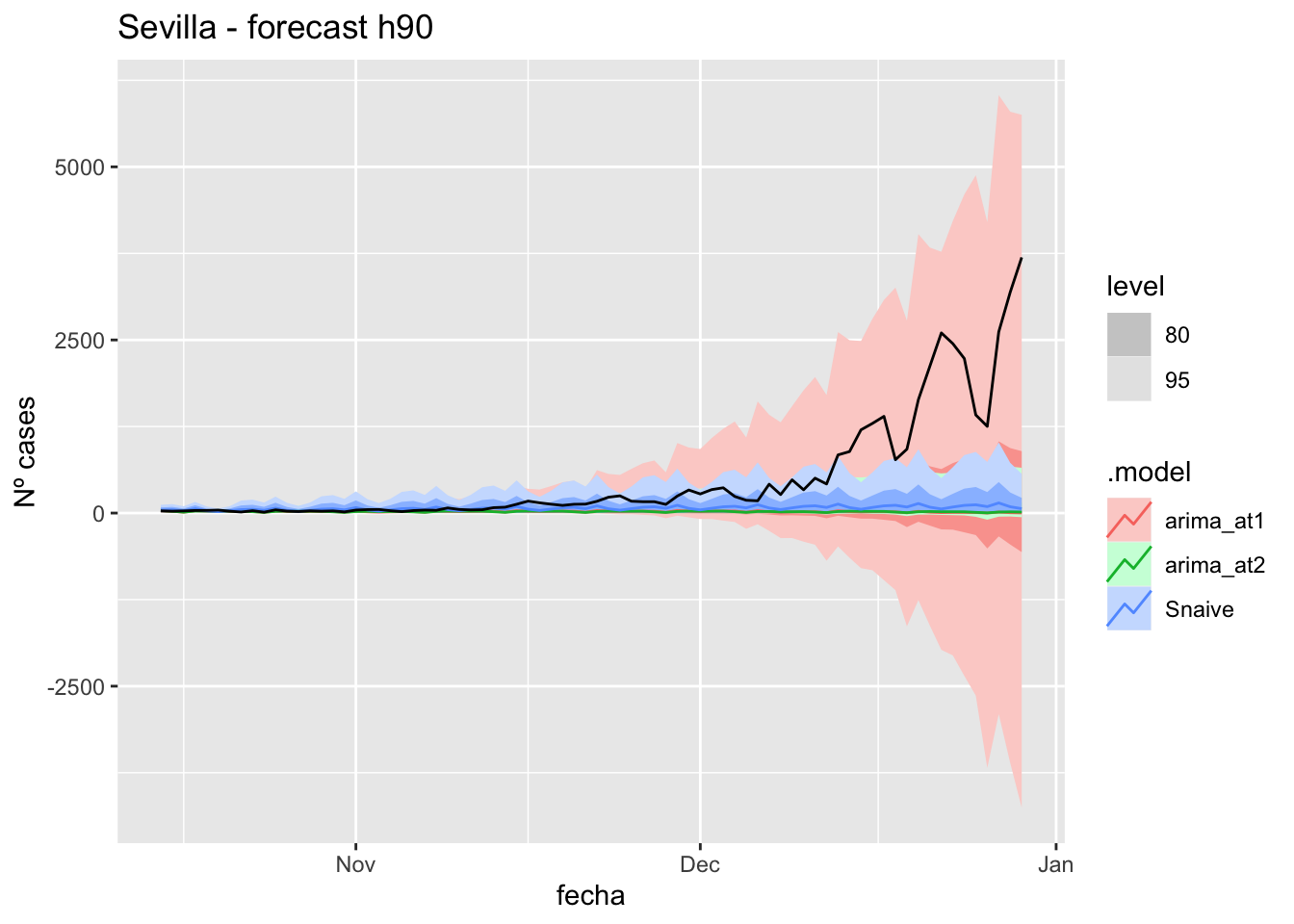
fc_h90 %>%
autoplot(
data_Sevilla %>%
filter(fecha <= as.Date("2021-10-14", format = "%Y-%m-%d")+days(90) &
fecha > as.Date("2021-07-01", format = "%Y-%m-%d"))
) +
labs(y = "Nº cases", title = "Sevilla - forecast h90")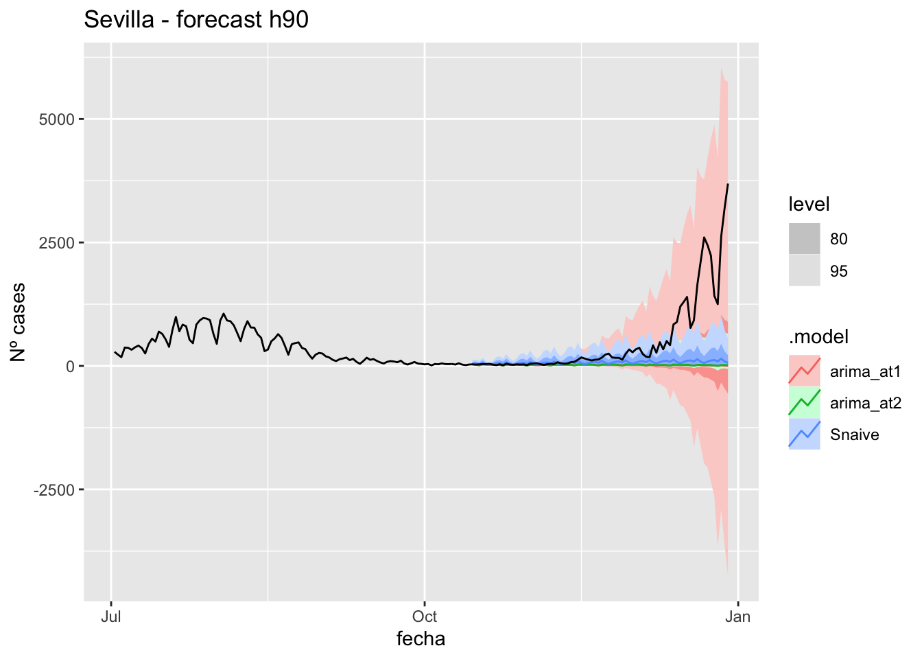
# Accuracy
fabletools::accuracy(fc_h90, data_Sevilla)# A tibble: 3 × 11
.model provincia .type ME RMSE MAE MPE MAPE MASE RMSSE ACF1
<chr> <chr> <chr> <dbl> <dbl> <dbl> <dbl> <dbl> <dbl> <dbl> <dbl>
1 arima_at1 Sevilla Test 486. 948. 487. 68.6 69.9 4.81 6.01 0.845
2 arima_at2 Sevilla Test 485. 945. 486. 67.3 70.6 4.80 5.99 0.845
3 Snaive Sevilla Test 436. 908. 449. 22.7 70.6 4.44 5.76 0.839Middel of sixth epidemiological period
Asturias
data_asturias <- covid_data %>%
filter(provincia == "Asturias") %>%
filter(fecha > as.Date("2020-06-14", format = "%Y-%m-%d")) %>%
select(provincia, fecha, num_casos, tmed, mob_flujo) %>%
drop_na() %>%
as_tsibble(key = provincia, index = fecha)
data_asturias# A tsibble: 563 x 5 [1D]
# Key: provincia [1]
provincia fecha num_casos tmed mob_flujo
<chr> <date> <dbl> <dbl> <dbl>
1 Asturias 2020-06-15 0 16 19.4
2 Asturias 2020-06-16 1 15.6 19.5
3 Asturias 2020-06-17 0 15.6 19.7
4 Asturias 2020-06-18 0 15.1 20.5
5 Asturias 2020-06-19 0 14.8 21.0
6 Asturias 2020-06-20 0 16.8 19.8
7 Asturias 2020-06-21 0 18.2 20.2
8 Asturias 2020-06-22 0 18.2 20.6
9 Asturias 2020-06-23 0 20 21.1
10 Asturias 2020-06-24 0 18.2 21.5
# … with 553 more rowsdata_asturias_train <- data_asturias %>%
filter(fecha <= as.Date("2021-12-10", format = "%Y-%m-%d"))
summary(data_asturias_train$fecha) Min. 1st Qu. Median Mean 3rd Qu. Max.
"2020-06-15" "2020-10-28" "2021-03-13" "2021-03-13" "2021-07-27" "2021-12-10" data_asturias_test <- data_asturias %>%
filter(fecha > as.Date("2021-12-10", format = "%Y-%m-%d"))
summary(data_asturias_test$fecha) Min. 1st Qu. Median Mean 3rd Qu. Max.
"2021-12-11" "2021-12-15" "2021-12-20" "2021-12-20" "2021-12-24" "2021-12-29" # Lamba for num_casos
lambda_asturias_casos <- data_asturias %>%
features(num_casos, features = guerrero) %>%
pull(lambda_guerrero)
lambda_asturias_casos[1] 0.2493395# Lamba for average temp
lambda_asturias_tmed <- data_asturias %>%
features(tmed, features = guerrero) %>%
pull(lambda_guerrero)
lambda_asturias_tmed[1] 1.142823# Lamba for mobility
lambda_asturias_mobil <- data_asturias %>%
features(mob_flujo, features = guerrero) %>%
pull(lambda_guerrero)
lambda_asturias_mobil[1] 1.459993fit_model <- data_asturias_train %>%
model(
arima_at1 = ARIMA(box_cox(num_casos, lambda_asturias_casos) ~
box_cox(tmed, lambda_asturias_tmed) +
box_cox(mob_flujo, lambda_asturias_mobil)),
arima_at2 = ARIMA(box_cox(num_casos, lambda_asturias_casos) ~
box_cox(tmed, lambda_asturias_tmed) +
box_cox(mob_flujo, lambda_asturias_mobil),
stepwise = FALSE, approx = FALSE),
Snaive = SNAIVE(box_cox(num_casos, lambda_asturias_casos))
)
# Show and report model
fit_model# A mable: 1 x 4
# Key: provincia [1]
provincia arima_at1
<chr> <model>
1 Asturias <LM w/ ARIMA(2,0,0)(2,1,1)[7] errors>
# … with 2 more variables: arima_at2 <model>, Snaive <model>glance(fit_model)# A tibble: 3 × 9
provincia .model sigma2 log_lik AIC AICc BIC ar_roots ma_roots
<chr> <chr> <dbl> <dbl> <dbl> <dbl> <dbl> <list> <list>
1 Asturias arima_at1 1.00 -765. 1545. 1546. 1580. <cpl [16]> <cpl [7]>
2 Asturias arima_at2 0.981 -757. 1534. 1535. 1577. <cpl [9]> <cpl [15]>
3 Asturias Snaive 2.69 NA NA NA NA <NULL> <NULL> fit_model %>%
pivot_longer(-provincia,
names_to = ".model",
values_to = "orders") %>%
left_join(glance(fit_model), by = c("provincia", ".model")) %>%
arrange(AICc) %>%
select(.model:BIC)# A mable: 3 x 7
# Key: .model [3]
.model orders sigma2 log_lik AIC AICc BIC
<chr> <model> <dbl> <dbl> <dbl> <dbl> <dbl>
1 arima_… <LM w/ ARIMA(2,0,1)(1,1,2)[7] errors> 0.981 -757. 1534. 1535. 1577.
2 arima_… <LM w/ ARIMA(2,0,0)(2,1,1)[7] errors> 1.00 -765. 1545. 1546. 1580.
3 Snaive <SNAIVE> 2.69 NA NA NA NA # We use a Ljung-Box test >> large p-value, confirms residuals are similar / considered to white noise
fit_model %>%
select(Snaive) %>%
gg_tsresiduals()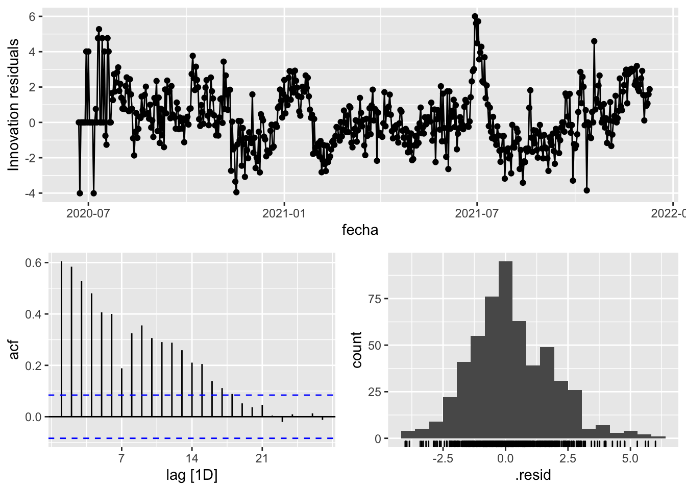
fit_model %>%
select(arima_at1) %>%
gg_tsresiduals()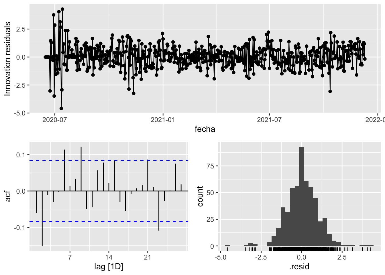
fit_model %>%
select(arima_at2) %>%
gg_tsresiduals()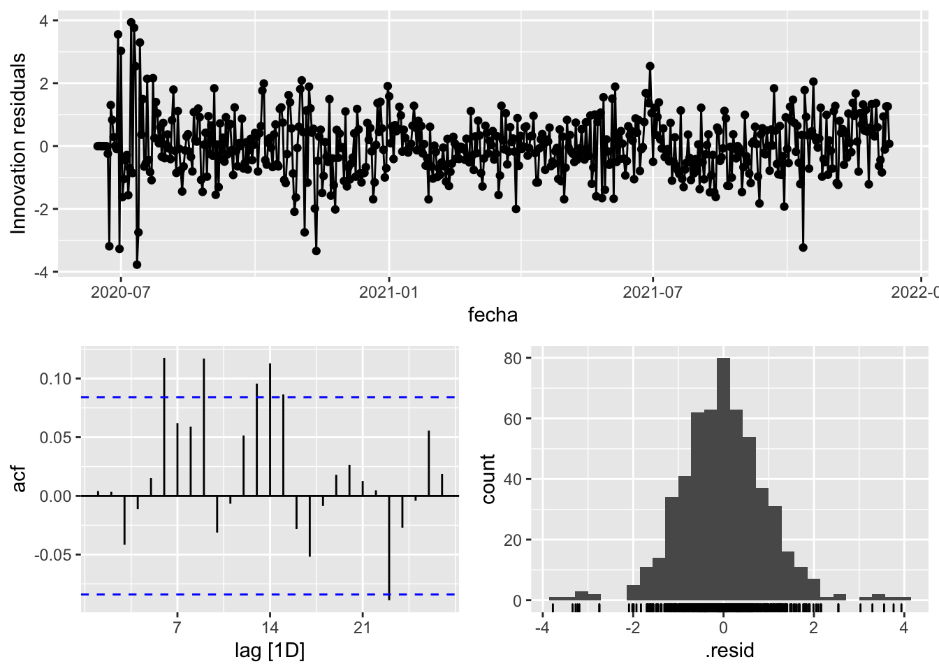
augment(fit_model) %>%
features(.innov, ljung_box, lag=7)# A tibble: 3 × 4
provincia .model lb_stat lb_pvalue
<chr> <chr> <dbl> <dbl>
1 Asturias arima_at1 22.4 0.00217
2 Asturias arima_at2 10.9 0.141
3 Asturias Snaive 855. 0 augment(fit_model) %>%
features(.innov, ljung_box, lag=14)# A tibble: 3 × 4
provincia .model lb_stat lb_pvalue
<chr> <chr> <dbl> <dbl>
1 Asturias arima_at1 39.3 0.000327
2 Asturias arima_at2 34.8 0.00159
3 Asturias Snaive 1188. 0 augment(fit_model) %>%
features(.innov, ljung_box, lag=21)# A tibble: 3 × 4
provincia .model lb_stat lb_pvalue
<chr> <chr> <dbl> <dbl>
1 Asturias arima_at1 50.0 0.000366
2 Asturias arima_at2 41.6 0.00466
3 Asturias Snaive 1236. 0 augment(fit_model) %>%
features(.innov, ljung_box, lag=57)# A tibble: 3 × 4
provincia .model lb_stat lb_pvalue
<chr> <chr> <dbl> <dbl>
1 Asturias arima_at1 79.5 0.0260
2 Asturias arima_at2 70.9 0.102
3 Asturias Snaive 1339. 0 # To predict future values of infections, we need to pass the model future/prediction values of the complementary variables tmed and mobility
# We are going to select those from the test dataset
data_fc_h7 <- data_asturias_test %>%
select(-num_casos) %>%
slice(1:7)
data_fc_h14 <- data_asturias_test %>%
select(-num_casos) %>%
slice(1:14)
data_fc_h21 <- data_asturias_test %>%
select(-num_casos) %>%
slice(1:21)
data_fc_h57 <- data_asturias_test %>%
select(-num_casos) %>%
slice(1:57)# Significant spikes out of 30 is still consistent with white noise
# To be sure, use a Ljung-Box test, which has a large p-value, confirming that
# the residuals are similar to white noise.
# Note that the alternative models also passed this test.
#
# Forecast
fc_h7 <- fabletools::forecast(fit_model, new_data = data_fc_h7)
fc_h14 <- fabletools::forecast(fit_model, new_data = data_fc_h14)
fc_h21 <- fabletools::forecast(fit_model, new_data = data_fc_h21)
fc_h57 <- fabletools::forecast(fit_model, new_data = data_fc_h57)7 days
# Plots
fc_h7 %>%
autoplot(
data_asturias_test %>%
filter(fecha <= as.Date("2021-12-10", format = "%Y-%m-%d")+days(7))
) +
labs(y = "Nº cases", title = "Asturias - forecast h7")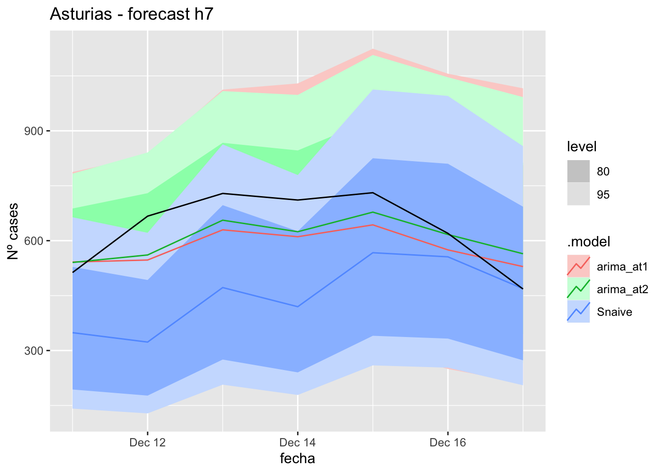
fc_h7 %>%
autoplot(
data_asturias %>%
filter(fecha <= as.Date("2021-12-10", format = "%Y-%m-%d")+days(7) &
fecha > as.Date("2021-10-01", format = "%Y-%m-%d"))
) +
labs(y = "Nº cases", title = "Asturias - forecast h7")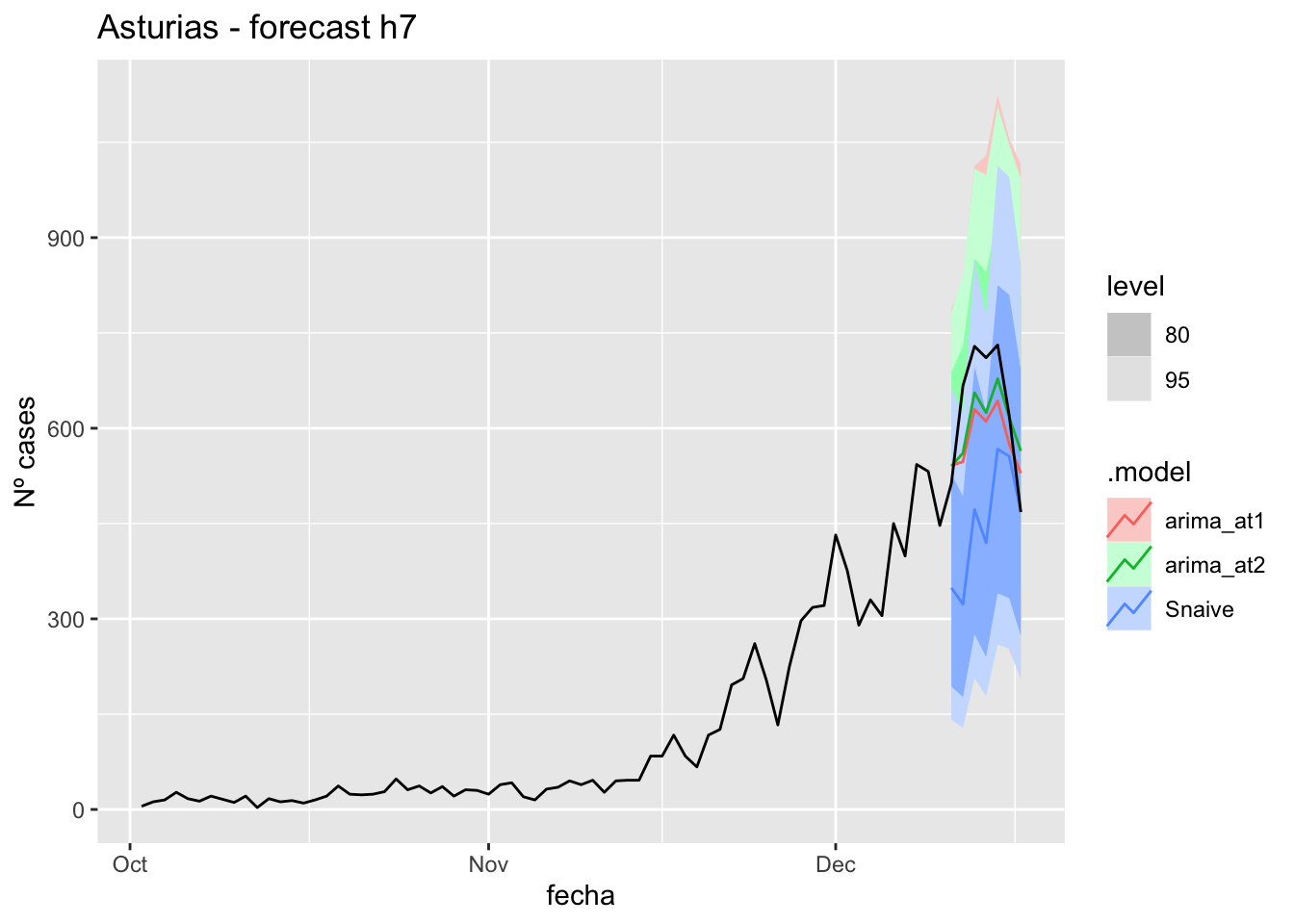
# Accuracy
fabletools::accuracy(fc_h7, data_asturias)# A tibble: 3 × 11
.model provincia .type ME RMSE MAE MPE MAPE MASE RMSSE ACF1
<chr> <chr> <chr> <dbl> <dbl> <dbl> <dbl> <dbl> <dbl> <dbl> <dbl>
1 arima_at1 Asturias Test 51.8 83.3 77.5 6.62 12.0 1.55 1.02 0.0778
2 arima_at2 Asturias Test 28.3 72.6 63.7 2.85 10.3 1.27 0.890 0.182
3 Snaive Asturias Test 183. 216. 184. 27.5 27.5 3.67 2.65 0.424 14 days
# Plots
fc_h14 %>%
autoplot(
data_asturias_test %>%
filter(fecha <= as.Date("2021-12-10", format = "%Y-%m-%d")+days(14))
) +
labs(y = "Nº cases", title = "Asturias - forecast h14")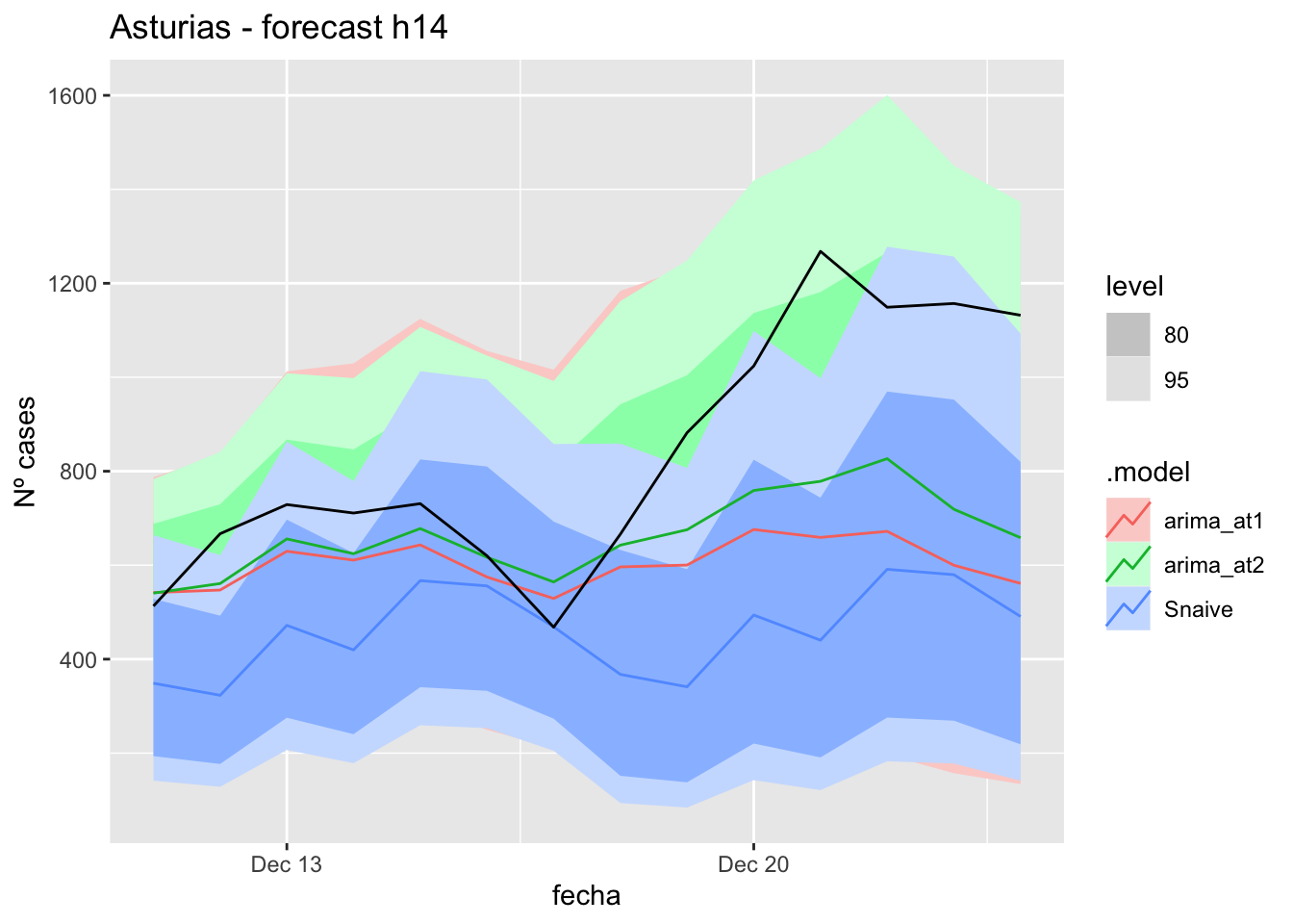
fc_h14 %>%
autoplot(
data_asturias %>%
filter(fecha <= as.Date("2021-12-10", format = "%Y-%m-%d")+days(14) &
fecha > as.Date("2021-10-01", format = "%Y-%m-%d"))
) +
labs(y = "Nº cases", title = "Asturias - forecast h14")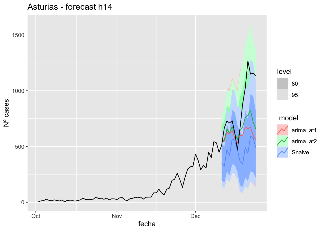
# Accuracy
fabletools::accuracy(fc_h14, data_asturias)# A tibble: 3 × 11
.model provincia .type ME RMSE MAE MPE MAPE MASE RMSSE ACF1
<chr> <chr> <chr> <dbl> <dbl> <dbl> <dbl> <dbl> <dbl> <dbl> <dbl>
1 arima_at1 Asturias Test 234. 326. 247. 22.2 24.9 4.93 4.00 0.739
2 arima_at2 Asturias Test 173. 255. 190. 15.6 19.4 3.80 3.12 0.688
3 Snaive Asturias Test 375. 442. 376. 40.8 40.8 7.50 5.41 0.66921 days
# Plots
fc_h21 %>%
autoplot(
data_asturias_test %>%
filter(fecha <= as.Date("2021-12-10", format = "%Y-%m-%d")+days(21))
) +
labs(y = "Nº cases", title = "Asturias - forecast h21")
fc_h21 %>%
autoplot(
data_asturias %>%
filter(fecha <= as.Date("2021-12-10", format = "%Y-%m-%d")+days(21) &
fecha > as.Date("2021-10-01", format = "%Y-%m-%d"))
) +
labs(y = "Nº cases", title = "Asturias - forecast h21")
# Accuracy
fabletools::accuracy(fc_h21, data_asturias)# A tibble: 3 × 11
.model provincia .type ME RMSE MAE MPE MAPE MASE RMSSE ACF1
<chr> <chr> <chr> <dbl> <dbl> <dbl> <dbl> <dbl> <dbl> <dbl> <dbl>
1 arima_at1 Asturias Test 512. 750. 522. 33.1 35.1 10.4 9.20 0.794
2 arima_at2 Asturias Test 424. 651. 437. 26.0 28.7 8.72 7.97 0.787
3 Snaive Asturias Test 670. 879. 670. 49.8 49.8 13.4 10.8 0.80657 days
# Plots
fc_h57 %>%
autoplot(
data_asturias_test %>%
filter(fecha <= as.Date("2021-12-10", format = "%Y-%m-%d")+days(57))
) +
labs(y = "Nº cases", title = "Asturias - forecast h57")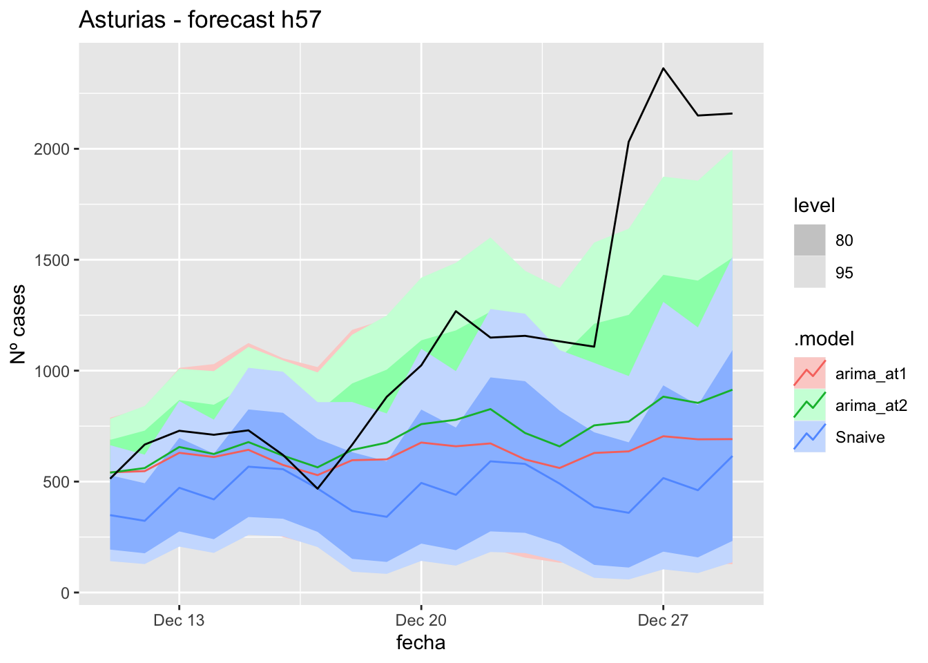
fc_h57 %>%
autoplot(
data_asturias %>%
filter(fecha <= as.Date("2021-12-10", format = "%Y-%m-%d")+days(57) &
fecha > as.Date("2021-10-01", format = "%Y-%m-%d"))
) +
labs(y = "Nº cases", title = "Asturias - forecast h57")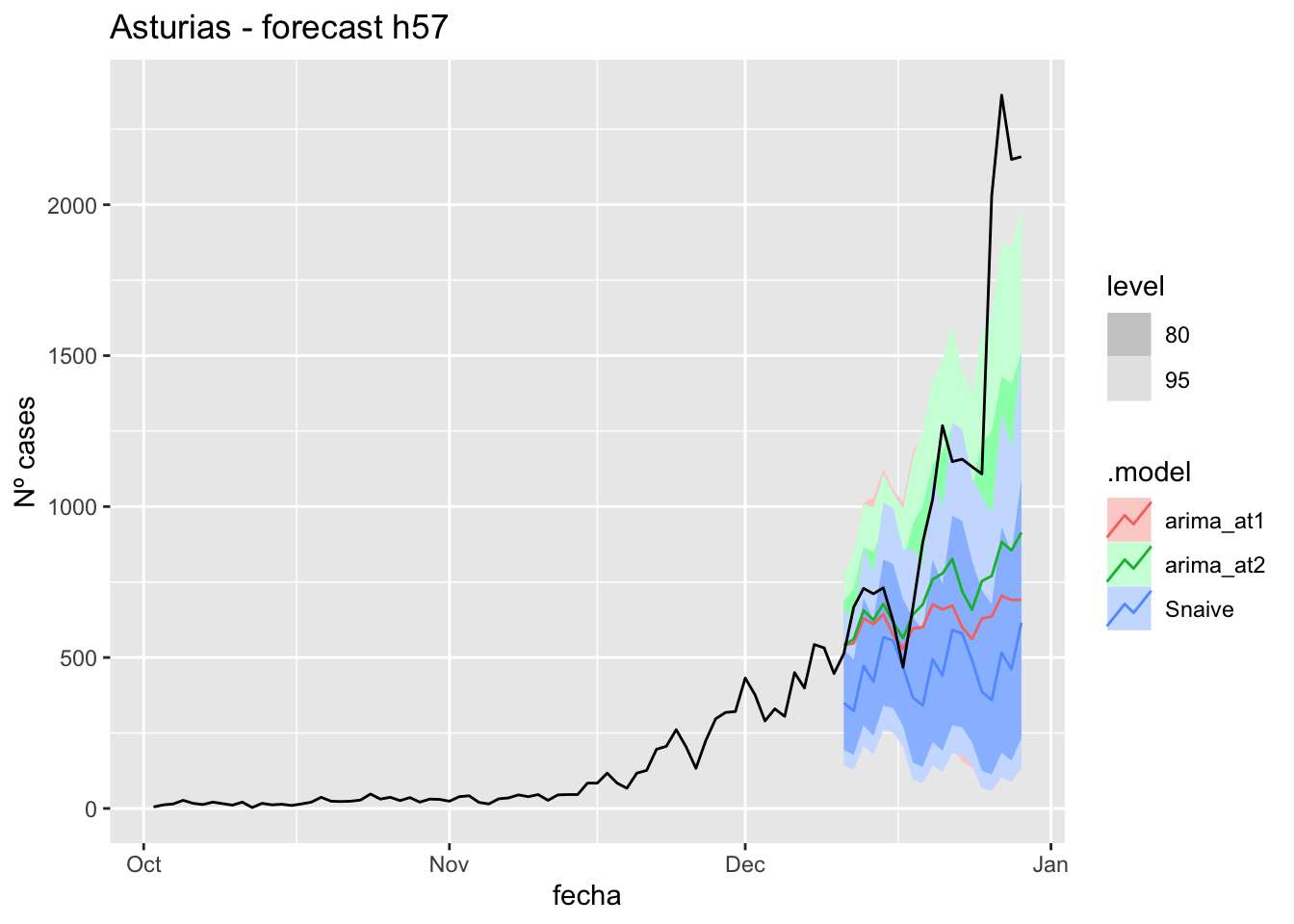
# Accuracy
fabletools::accuracy(fc_h57, data_asturias)# A tibble: 3 × 11
.model provincia .type ME RMSE MAE MPE MAPE MASE RMSSE ACF1
<chr> <chr> <chr> <dbl> <dbl> <dbl> <dbl> <dbl> <dbl> <dbl> <dbl>
1 arima_at1 Asturias Test 512. 750. 522. 33.1 35.1 10.4 9.20 0.794
2 arima_at2 Asturias Test 424. 651. 437. 26.0 28.7 8.72 7.97 0.787
3 Snaive Asturias Test 670. 879. 670. 49.8 49.8 13.4 10.8 0.806Barcelona
data_Barcelona <- covid_data %>%
filter(provincia == "Barcelona") %>%
filter(fecha > as.Date("2020-06-14", format = "%Y-%m-%d")) %>%
select(provincia, fecha, num_casos, tmed, mob_flujo) %>%
drop_na() %>%
as_tsibble(key = provincia, index = fecha)
data_Barcelona# A tsibble: 563 x 5 [1D]
# Key: provincia [1]
provincia fecha num_casos tmed mob_flujo
<chr> <date> <dbl> <dbl> <dbl>
1 Barcelona 2020-06-15 62 21.2 22.0
2 Barcelona 2020-06-16 66 20.8 22.6
3 Barcelona 2020-06-17 70 20.3 23.2
4 Barcelona 2020-06-18 68 18.8 23.2
5 Barcelona 2020-06-19 65 20.4 23.9
6 Barcelona 2020-06-20 53 21.8 21.5
7 Barcelona 2020-06-21 38 22.8 20.5
8 Barcelona 2020-06-22 69 23.8 19.5
9 Barcelona 2020-06-23 95 23.4 18.5
10 Barcelona 2020-06-24 44 23.6 17.5
# … with 553 more rowsdata_Barcelona_train <- data_Barcelona %>%
filter(fecha <= as.Date("2021-12-10", format = "%Y-%m-%d"))
summary(data_Barcelona_train$fecha) Min. 1st Qu. Median Mean 3rd Qu. Max.
"2020-06-15" "2020-10-28" "2021-03-13" "2021-03-13" "2021-07-27" "2021-12-10" data_Barcelona_test <- data_Barcelona %>%
filter(fecha > as.Date("2021-12-10", format = "%Y-%m-%d"))
summary(data_Barcelona_test$fecha) Min. 1st Qu. Median Mean 3rd Qu. Max.
"2021-12-11" "2021-12-15" "2021-12-20" "2021-12-20" "2021-12-24" "2021-12-29" # Lamba for num_casos
lambda_Barcelona_casos <- data_Barcelona %>%
features(num_casos, features = guerrero) %>%
pull(lambda_guerrero)
lambda_Barcelona_casos[1] 0.07878312# Lamba for average temp
lambda_Barcelona_tmed <- data_Barcelona %>%
features(tmed, features = guerrero) %>%
pull(lambda_guerrero)
lambda_Barcelona_tmed[1] 1.143918# Lamba for mobility
lambda_Barcelona_mobil <- data_Barcelona %>%
features(mob_flujo, features = guerrero) %>%
pull(lambda_guerrero)
lambda_Barcelona_mobil[1] 1.072959fit_model <- data_Barcelona_train %>%
model(
arima_at1 = ARIMA(box_cox(num_casos, lambda_Barcelona_casos) ~
box_cox(tmed, lambda_Barcelona_tmed) +
box_cox(mob_flujo, lambda_Barcelona_mobil)),
arima_at2 = ARIMA(box_cox(num_casos, lambda_Barcelona_casos) ~
box_cox(tmed, lambda_Barcelona_tmed) +
box_cox(mob_flujo, lambda_Barcelona_mobil),
stepwise = FALSE, approx = FALSE),
Snaive = SNAIVE(box_cox(num_casos, lambda_Barcelona_casos))
)
# Show and report model
fit_model# A mable: 1 x 4
# Key: provincia [1]
provincia arima_at1
<chr> <model>
1 Barcelona <LM w/ ARIMA(1,0,2)(0,1,0)[7] errors>
# … with 2 more variables: arima_at2 <model>, Snaive <model>glance(fit_model)# A tibble: 3 × 9
provincia .model sigma2 log_lik AIC AICc BIC ar_roots ma_roots
<chr> <chr> <dbl> <dbl> <dbl> <dbl> <dbl> <list> <list>
1 Barcelona arima_at1 0.156 -261. 533. 533. 559. <cpl [1]> <cpl [2]>
2 Barcelona arima_at2 0.116 -185. 387. 388. 426. <cpl [4]> <cpl [8]>
3 Barcelona Snaive 0.413 NA NA NA NA <NULL> <NULL> fit_model %>%
pivot_longer(-provincia,
names_to = ".model",
values_to = "orders") %>%
left_join(glance(fit_model), by = c("provincia", ".model")) %>%
arrange(AICc) %>%
select(.model:BIC)# A mable: 3 x 7
# Key: .model [3]
.model orders sigma2 log_lik AIC AICc BIC
<chr> <model> <dbl> <dbl> <dbl> <dbl> <dbl>
1 arima_… <LM w/ ARIMA(4,0,1)(0,1,1)[7] errors> 0.116 -185. 387. 388. 426.
2 arima_… <LM w/ ARIMA(1,0,2)(0,1,0)[7] errors> 0.156 -261. 533. 533. 559.
3 Snaive <SNAIVE> 0.413 NA NA NA NA # We use a Ljung-Box test >> large p-value, confirms residuals are similar / considered to white noise
fit_model %>%
select(Snaive) %>%
gg_tsresiduals()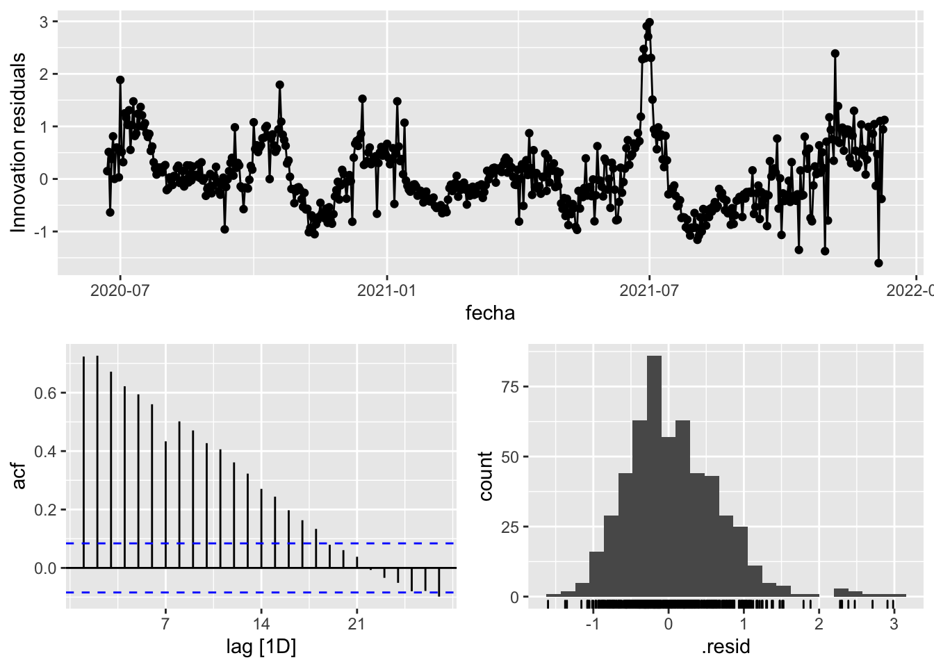
fit_model %>%
select(arima_at1) %>%
gg_tsresiduals()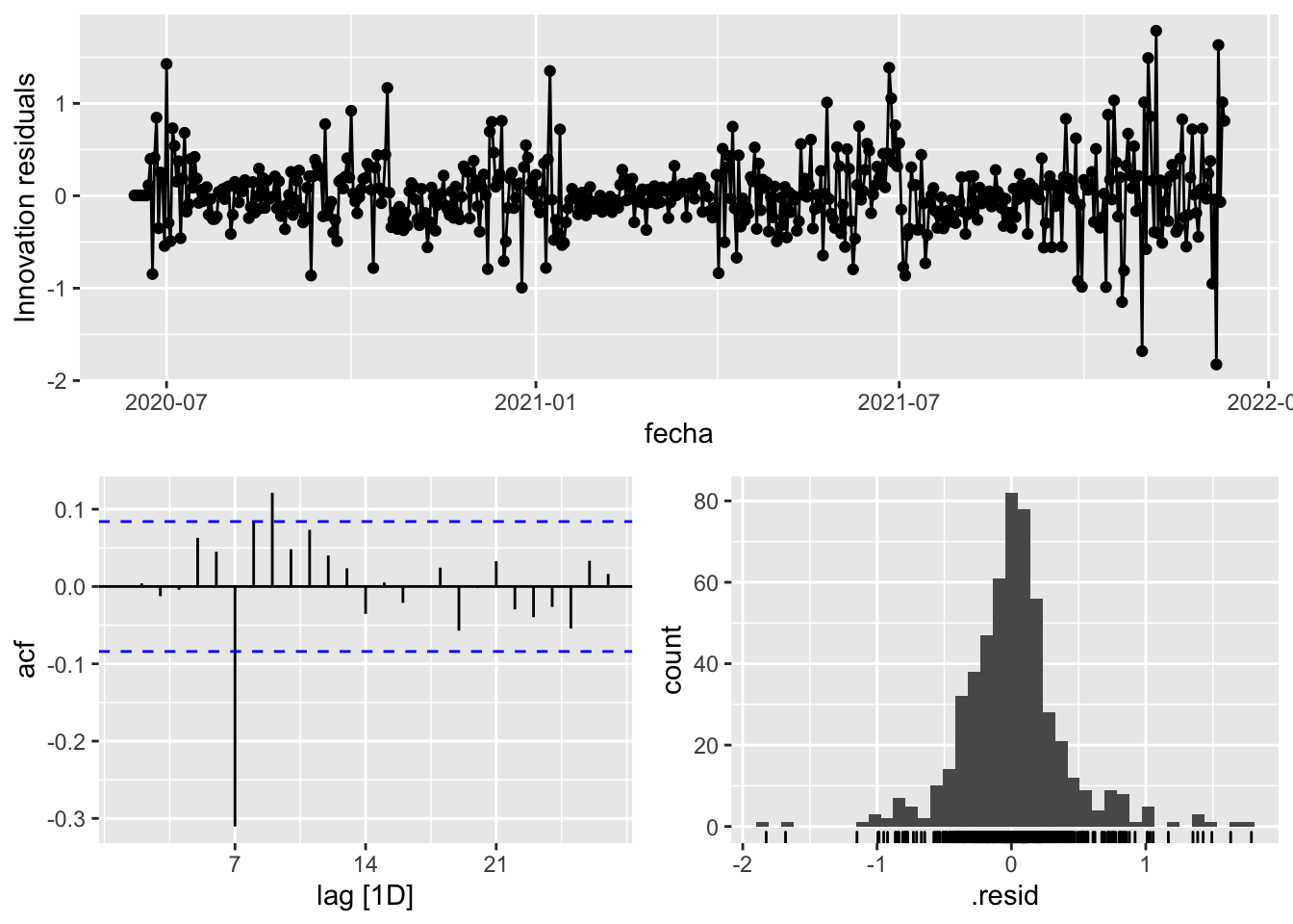
fit_model %>%
select(arima_at2) %>%
gg_tsresiduals()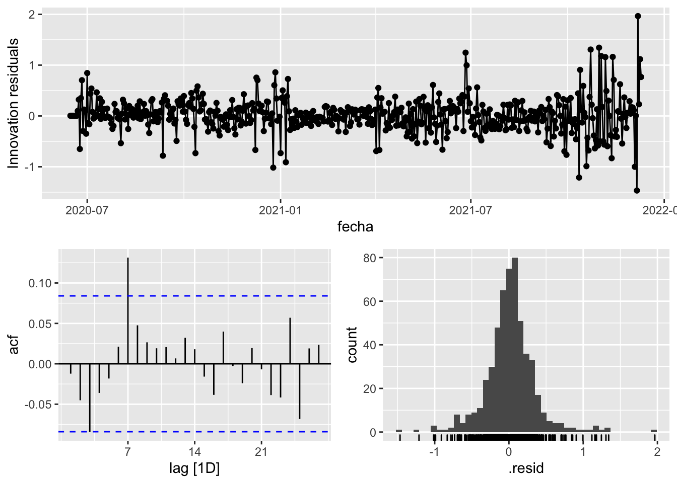
augment(fit_model) %>%
features(.innov, ljung_box, lag=7)# A tibble: 3 × 4
provincia .model lb_stat lb_pvalue
<chr> <chr> <dbl> <dbl>
1 Barcelona arima_at1 56.7 6.83e-10
2 Barcelona arima_at2 15.8 2.69e- 2
3 Barcelona Snaive 1489. 0 augment(fit_model) %>%
features(.innov, ljung_box, lag=14)# A tibble: 3 × 4
provincia .model lb_stat lb_pvalue
<chr> <chr> <dbl> <dbl>
1 Barcelona arima_at1 74.9 2.49e-10
2 Barcelona arima_at2 18.7 1.77e- 1
3 Barcelona Snaive 2109. 0 augment(fit_model) %>%
features(.innov, ljung_box, lag=21)# A tibble: 3 × 4
provincia .model lb_stat lb_pvalue
<chr> <chr> <dbl> <dbl>
1 Barcelona arima_at1 77.9 0.0000000178
2 Barcelona arima_at2 21.1 0.451
3 Barcelona Snaive 2195. 0 augment(fit_model) %>%
features(.innov, ljung_box, lag=57)# A tibble: 3 × 4
provincia .model lb_stat lb_pvalue
<chr> <chr> <dbl> <dbl>
1 Barcelona arima_at1 130. 0.000000142
2 Barcelona arima_at2 78.4 0.0314
3 Barcelona Snaive 2888. 0 # To predict future values of infections, we need to pass the model future/prediction values of the complementary variables tmed and mobility
# We are going to select those from the test dataset
data_fc_h7 <- data_Barcelona_test %>%
select(-num_casos) %>%
slice(1:7)
data_fc_h14 <- data_Barcelona_test %>%
select(-num_casos) %>%
slice(1:14)
data_fc_h21 <- data_Barcelona_test %>%
select(-num_casos) %>%
slice(1:21)
data_fc_h57 <- data_Barcelona_test %>%
select(-num_casos) %>%
slice(1:57)# Significant spikes out of 30 is still consistent with white noise
# To be sure, use a Ljung-Box test, which has a large p-value, confirming that
# the residuals are similar to white noise.
# Note that the alternative models also passed this test.
#
# Forecast
fc_h7 <- fabletools::forecast(fit_model, new_data = data_fc_h7)
fc_h14 <- fabletools::forecast(fit_model, new_data = data_fc_h14)
fc_h21 <- fabletools::forecast(fit_model, new_data = data_fc_h21)
fc_h57 <- fabletools::forecast(fit_model, new_data = data_fc_h57)7 days
# Plots
fc_h7 %>%
autoplot(
data_Barcelona_test %>%
filter(fecha <= as.Date("2021-12-10", format = "%Y-%m-%d")+days(7))
) +
labs(y = "Nº cases", title = "Barcelona - forecast h7")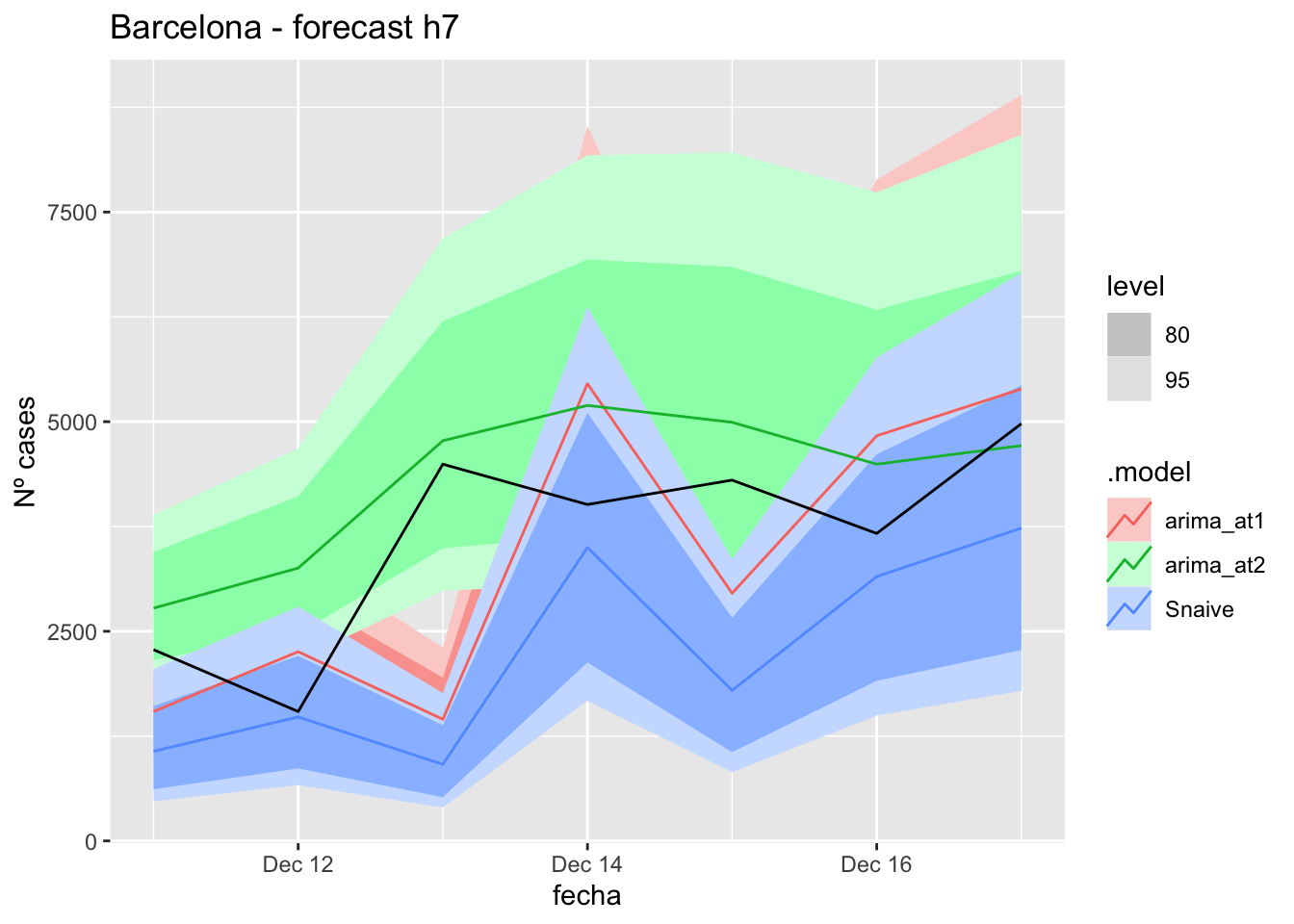
fc_h7 %>%
autoplot(
data_Barcelona %>%
filter(fecha <= as.Date("2021-12-10", format = "%Y-%m-%d")+days(7) &
fecha > as.Date("2021-10-01", format = "%Y-%m-%d"))
) +
labs(y = "Nº cases", title = "Barcelona - forecast h7")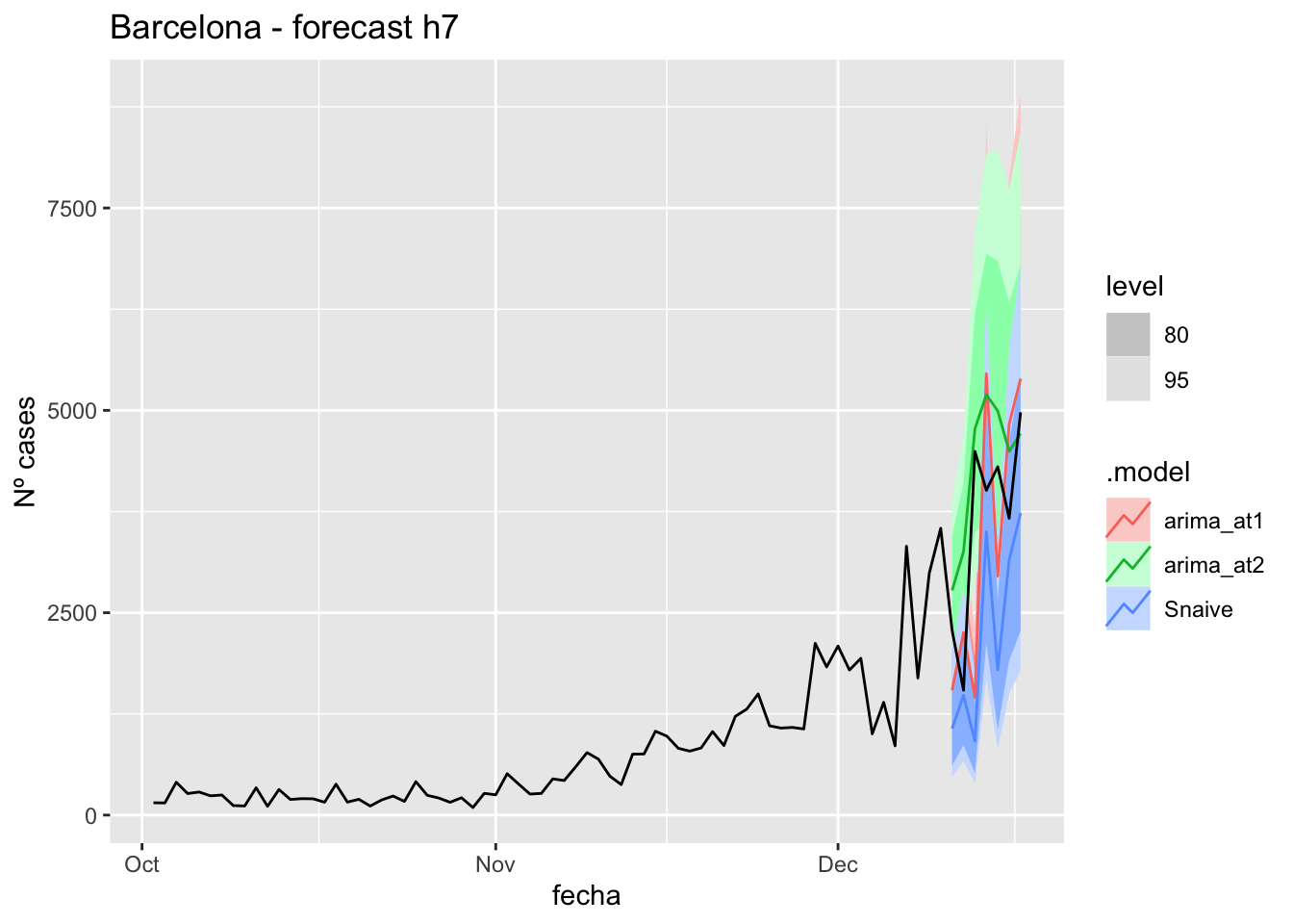
# Accuracy
fabletools::accuracy(fc_h7, data_Barcelona)# A tibble: 3 × 11
.model provincia .type ME RMSE MAE MPE MAPE MASE RMSSE ACF1
<chr> <chr> <chr> <dbl> <dbl> <dbl> <dbl> <dbl> <dbl> <dbl> <dbl>
1 arima_at1 Barcelona Test 200. 1499. 1266. 1.31 36.2 3.42 2.32 -0.671
2 arima_at2 Barcelona Test -703. 916. 778. -28.8 30.3 2.10 1.42 -0.400
3 Snaive Barcelona Test 1377. 1799. 1377. 35.3 35.3 3.72 2.79 -0.68314 days
# Plots
fc_h14 %>%
autoplot(
data_Barcelona_test %>%
filter(fecha <= as.Date("2021-12-10", format = "%Y-%m-%d")+days(14))
) +
labs(y = "Nº cases", title = "Barcelona - forecast h14")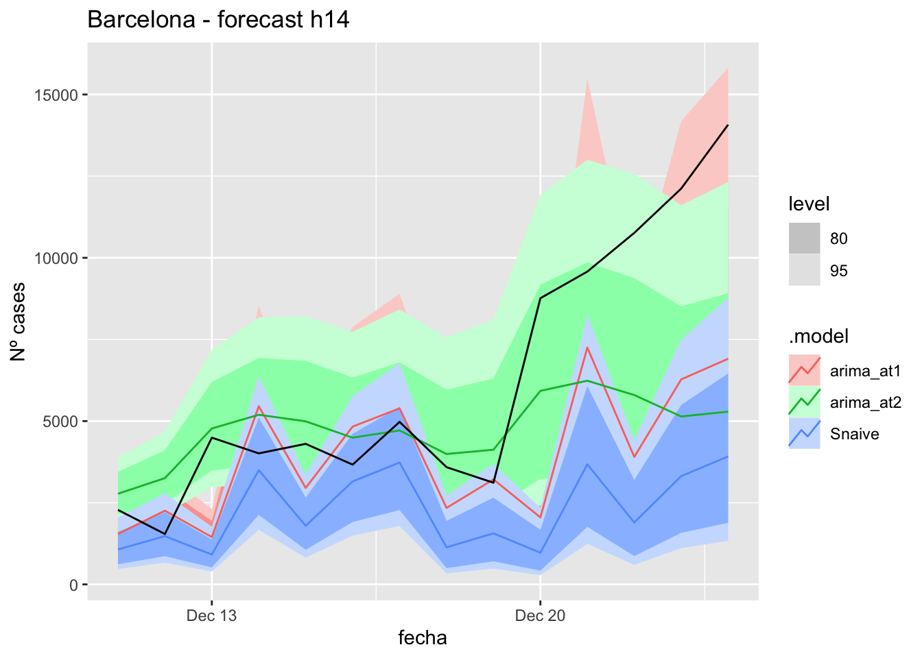
fc_h14 %>%
autoplot(
data_Barcelona %>%
filter(fecha <= as.Date("2021-12-10", format = "%Y-%m-%d")+days(14) &
fecha > as.Date("2021-10-01", format = "%Y-%m-%d"))
) +
labs(y = "Nº cases", title = "Barcelona - forecast h14")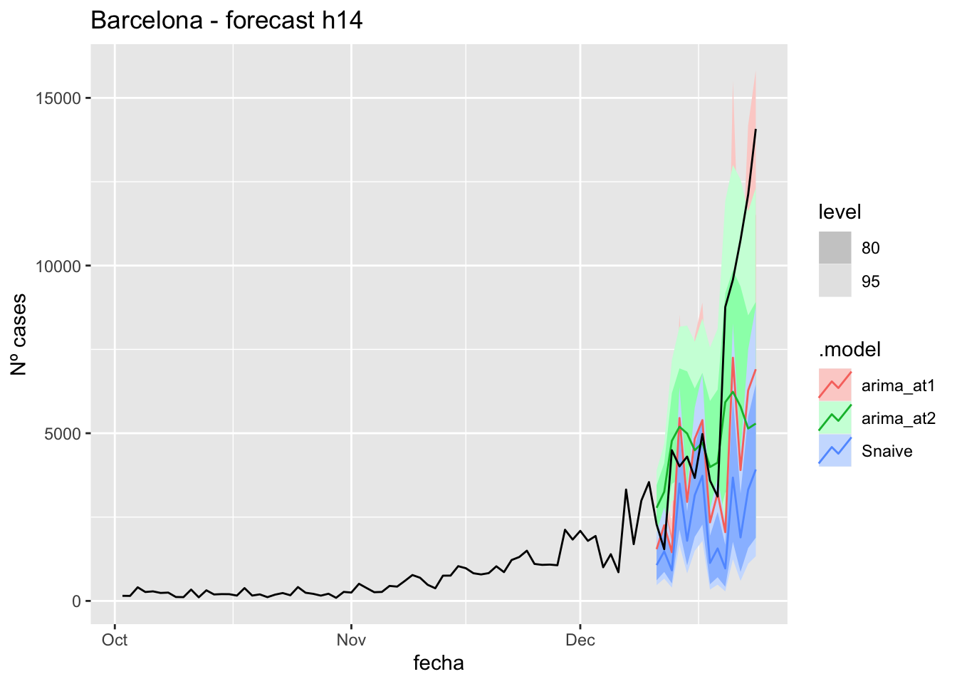
# Accuracy
fabletools::accuracy(fc_h14, data_Barcelona)# A tibble: 3 × 11
.model provincia .type ME RMSE MAE MPE MAPE MASE RMSSE ACF1
<chr> <chr> <chr> <dbl> <dbl> <dbl> <dbl> <dbl> <dbl> <dbl> <dbl>
1 arima_at1 Barcelona Test 2247. 3783. 2794. 21.7 39.7 7.55 5.86 0.340
2 arima_at2 Barcelona Test 1469. 3554. 2412. -0.849 34.9 6.52 5.50 0.696
3 Snaive Barcelona Test 3940. 5251. 3940. 53.1 53.1 10.7 8.13 0.60521 days
# Plots
fc_h21 %>%
autoplot(
data_Barcelona_test %>%
filter(fecha <= as.Date("2021-12-10", format = "%Y-%m-%d")+days(21))
) +
labs(y = "Nº cases", title = "Barcelona - forecast h21")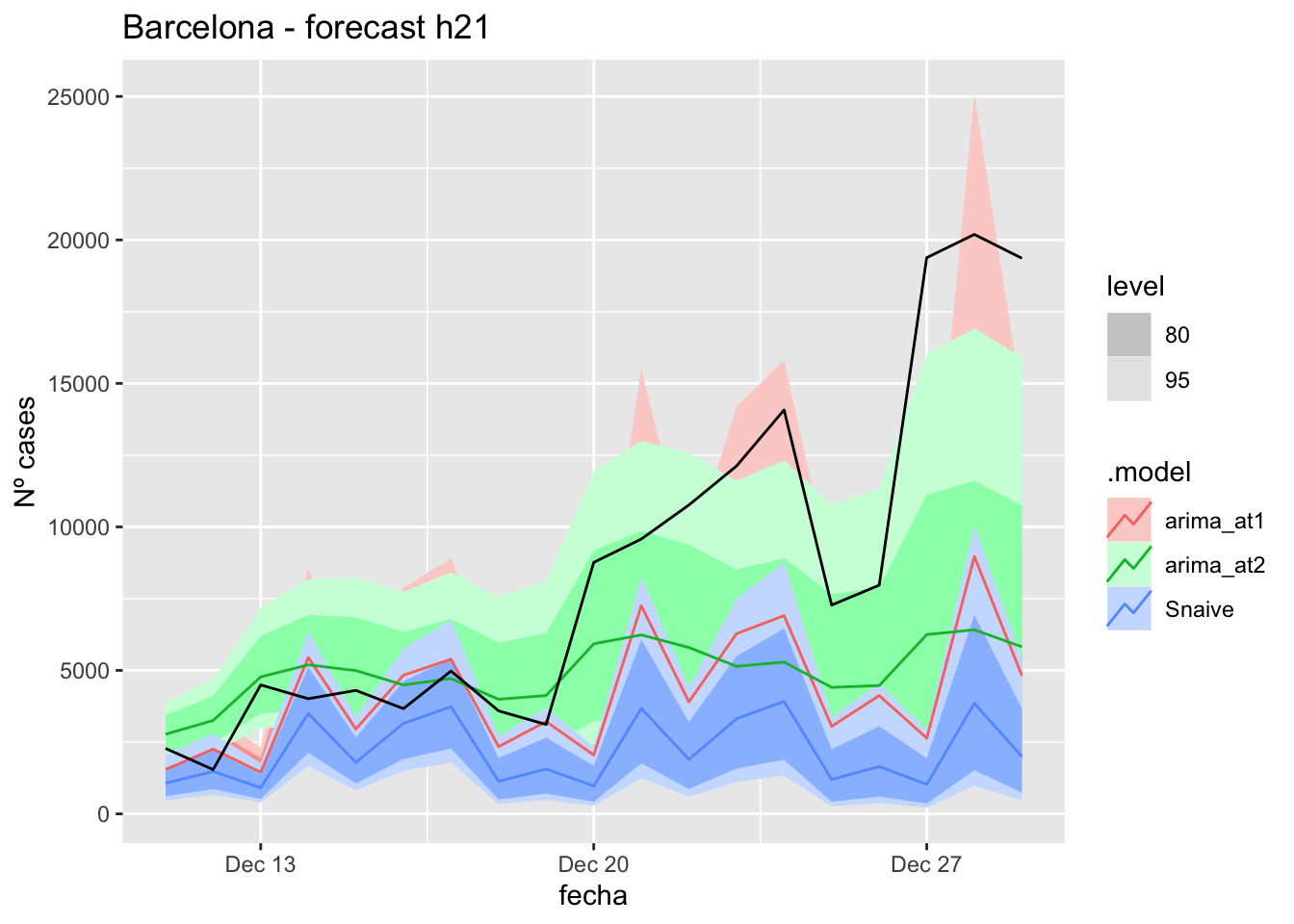
fc_h21 %>%
autoplot(
data_Barcelona %>%
filter(fecha <= as.Date("2021-12-10", format = "%Y-%m-%d")+days(21) &
fecha > as.Date("2021-10-01", format = "%Y-%m-%d"))
) +
labs(y = "Nº cases", title = "Barcelona - forecast h21")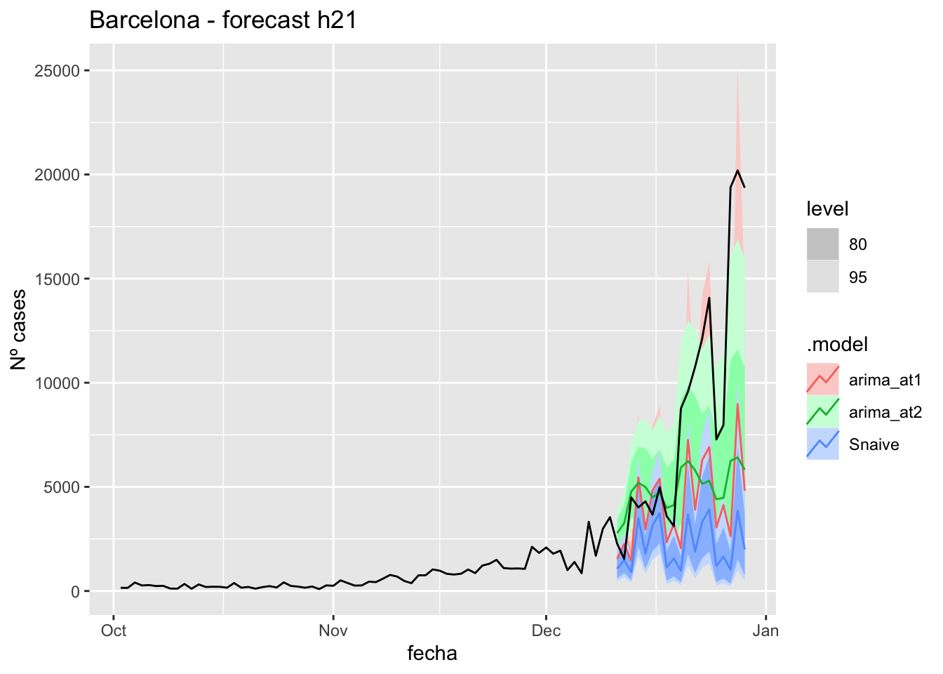
# Accuracy
fabletools::accuracy(fc_h21, data_Barcelona)# A tibble: 3 × 11
.model provincia .type ME RMSE MAE MPE MAPE MASE RMSSE ACF1
<chr> <chr> <chr> <dbl> <dbl> <dbl> <dbl> <dbl> <dbl> <dbl> <dbl>
1 arima_at1 Barcelona Test 4318. 6692. 4721. 33.0 46.3 12.8 10.4 0.518
2 arima_at2 Barcelona Test 3547. 6253. 4241. 14.6 41.0 11.5 9.68 0.726
3 Snaive Barcelona Test 6296. 8486. 6296. 61.6 61.6 17.0 13.1 0.67357 days
# Plots
fc_h57 %>%
autoplot(
data_Barcelona_test %>%
filter(fecha <= as.Date("2021-12-10", format = "%Y-%m-%d")+days(57))
) +
labs(y = "Nº cases", title = "Barcelona - forecast h57")
fc_h57 %>%
autoplot(
data_Barcelona %>%
filter(fecha <= as.Date("2021-12-10", format = "%Y-%m-%d")+days(57) &
fecha > as.Date("2021-10-01", format = "%Y-%m-%d"))
) +
labs(y = "Nº cases", title = "Barcelona - forecast h57")
# Accuracy
fabletools::accuracy(fc_h57, data_Barcelona)# A tibble: 3 × 11
.model provincia .type ME RMSE MAE MPE MAPE MASE RMSSE ACF1
<chr> <chr> <chr> <dbl> <dbl> <dbl> <dbl> <dbl> <dbl> <dbl> <dbl>
1 arima_at1 Barcelona Test 4318. 6692. 4721. 33.0 46.3 12.8 10.4 0.518
2 arima_at2 Barcelona Test 3547. 6253. 4241. 14.6 41.0 11.5 9.68 0.726
3 Snaive Barcelona Test 6296. 8486. 6296. 61.6 61.6 17.0 13.1 0.673Madrid
data_Madrid <- covid_data %>%
filter(provincia == "Madrid") %>%
filter(fecha > as.Date("2020-06-14", format = "%Y-%m-%d")) %>%
select(provincia, fecha, num_casos, tmed, mob_flujo) %>%
drop_na() %>%
as_tsibble(key = provincia, index = fecha)
data_Madrid# A tsibble: 563 x 5 [1D]
# Key: provincia [1]
provincia fecha num_casos tmed mob_flujo
<chr> <date> <dbl> <dbl> <dbl>
1 Madrid 2020-06-15 153 20.7 20.6
2 Madrid 2020-06-16 91 21 21.6
3 Madrid 2020-06-17 93 20.2 21.8
4 Madrid 2020-06-18 85 21.9 22.1
5 Madrid 2020-06-19 78 22.6 22.0
6 Madrid 2020-06-20 67 23.4 18.8
7 Madrid 2020-06-21 42 25 19.9
8 Madrid 2020-06-22 60 27.3 21.0
9 Madrid 2020-06-23 68 28.4 22.1
10 Madrid 2020-06-24 49 28 23.1
# … with 553 more rowsdata_Madrid_train <- data_Madrid %>%
filter(fecha <= as.Date("2021-12-10", format = "%Y-%m-%d"))
summary(data_Madrid_train$fecha) Min. 1st Qu. Median Mean 3rd Qu. Max.
"2020-06-15" "2020-10-28" "2021-03-13" "2021-03-13" "2021-07-27" "2021-12-10" data_Madrid_test <- data_Madrid %>%
filter(fecha > as.Date("2021-12-10", format = "%Y-%m-%d"))
summary(data_Madrid_test$fecha) Min. 1st Qu. Median Mean 3rd Qu. Max.
"2021-12-11" "2021-12-15" "2021-12-20" "2021-12-20" "2021-12-24" "2021-12-29" # Lamba for num_casos
lambda_Madrid_casos <- data_Madrid %>%
features(num_casos, features = guerrero) %>%
pull(lambda_guerrero)
lambda_Madrid_casos[1] 0.004154257# Lamba for average temp
lambda_Madrid_tmed <- data_Madrid %>%
features(tmed, features = guerrero) %>%
pull(lambda_guerrero)
lambda_Madrid_tmed[1] 0.9461578# Lamba for mobility
lambda_Madrid_mobil <- data_Madrid %>%
features(mob_flujo, features = guerrero) %>%
pull(lambda_guerrero)
lambda_Madrid_mobil[1] -0.01895186fit_model <- data_Madrid_train %>%
model(
arima_at1 = ARIMA(box_cox(num_casos, lambda_Madrid_casos) ~
box_cox(tmed, lambda_Madrid_tmed) +
box_cox(mob_flujo, lambda_Madrid_mobil)),
arima_at2 = ARIMA(box_cox(num_casos, lambda_Madrid_casos) ~
box_cox(tmed, lambda_Madrid_tmed) +
box_cox(mob_flujo, lambda_Madrid_mobil),
stepwise = FALSE, approx = FALSE),
Snaive = SNAIVE(box_cox(num_casos, lambda_Madrid_casos))
)
# Show and report model
fit_model# A mable: 1 x 4
# Key: provincia [1]
provincia arima_at1
<chr> <model>
1 Madrid <LM w/ ARIMA(2,0,1)(0,1,1)[7] errors>
# … with 2 more variables: arima_at2 <model>, Snaive <model>glance(fit_model)# A tibble: 3 × 9
provincia .model sigma2 log_lik AIC AICc BIC ar_roots ma_roots
<chr> <chr> <dbl> <dbl> <dbl> <dbl> <dbl> <list> <list>
1 Madrid arima_at1 0.0522 32.4 -50.8 -50.6 -20.8 <cpl [2]> <cpl [8]>
2 Madrid arima_at2 0.0497 46.3 -74.6 -74.2 -36.0 <cpl [2]> <cpl [9]>
3 Madrid Snaive 0.138 NA NA NA NA <NULL> <NULL> fit_model %>%
pivot_longer(-provincia,
names_to = ".model",
values_to = "orders") %>%
left_join(glance(fit_model), by = c("provincia", ".model")) %>%
arrange(AICc) %>%
select(.model:BIC)# A mable: 3 x 7
# Key: .model [3]
.model orders sigma2 log_lik AIC AICc BIC
<chr> <model> <dbl> <dbl> <dbl> <dbl> <dbl>
1 arima_… <LM w/ ARIMA(2,0,2)(0,1,1)[7] errors> 0.0497 46.3 -74.6 -74.2 -36.0
2 arima_… <LM w/ ARIMA(2,0,1)(0,1,1)[7] errors> 0.0522 32.4 -50.8 -50.6 -20.8
3 Snaive <SNAIVE> 0.138 NA NA NA NA # We use a Ljung-Box test >> large p-value, confirms residuals are similar / considered to white noise
fit_model %>%
select(Snaive) %>%
gg_tsresiduals()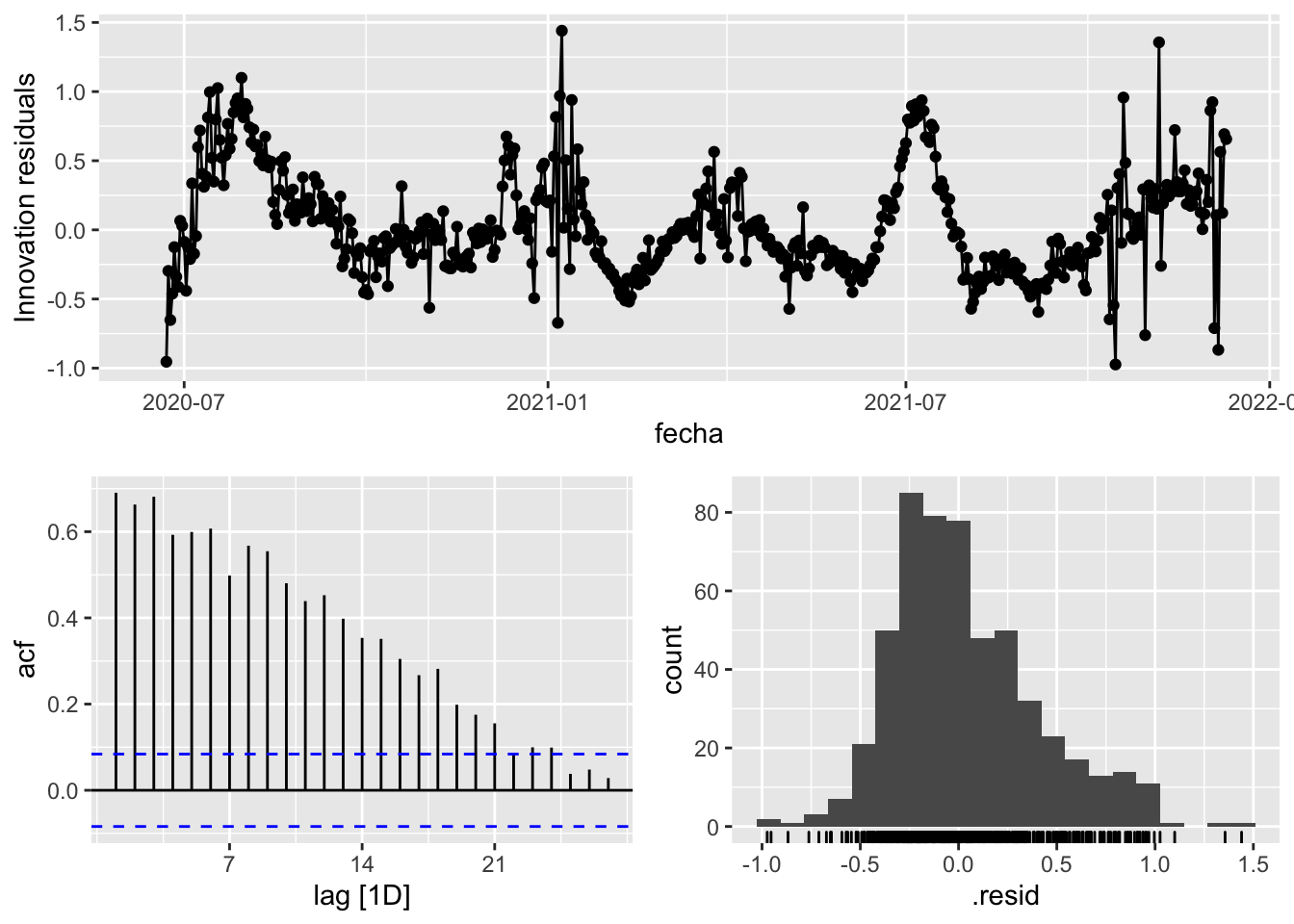
fit_model %>%
select(arima_at1) %>%
gg_tsresiduals()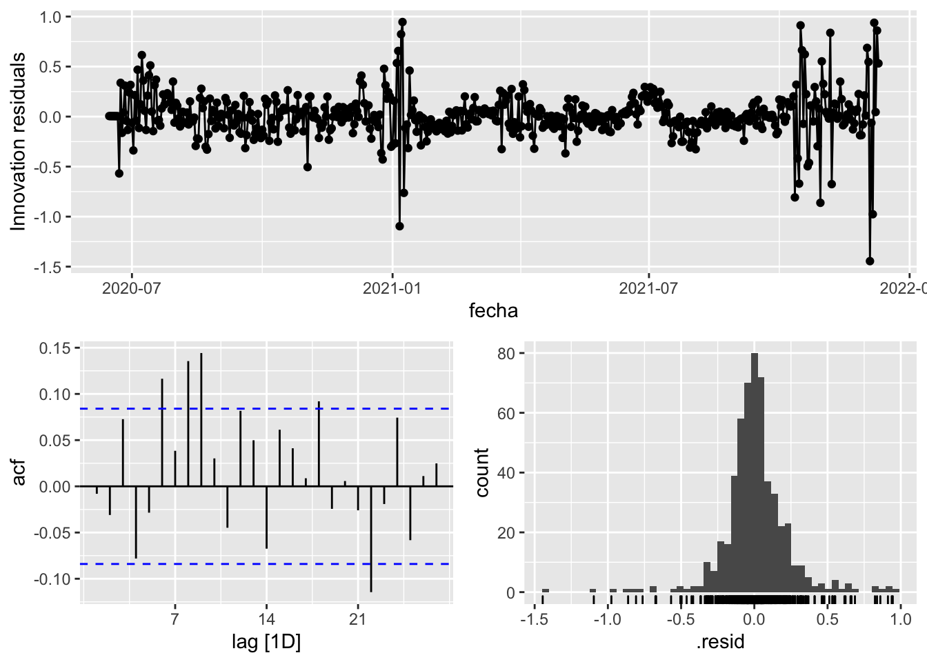
fit_model %>%
select(arima_at2) %>%
gg_tsresiduals()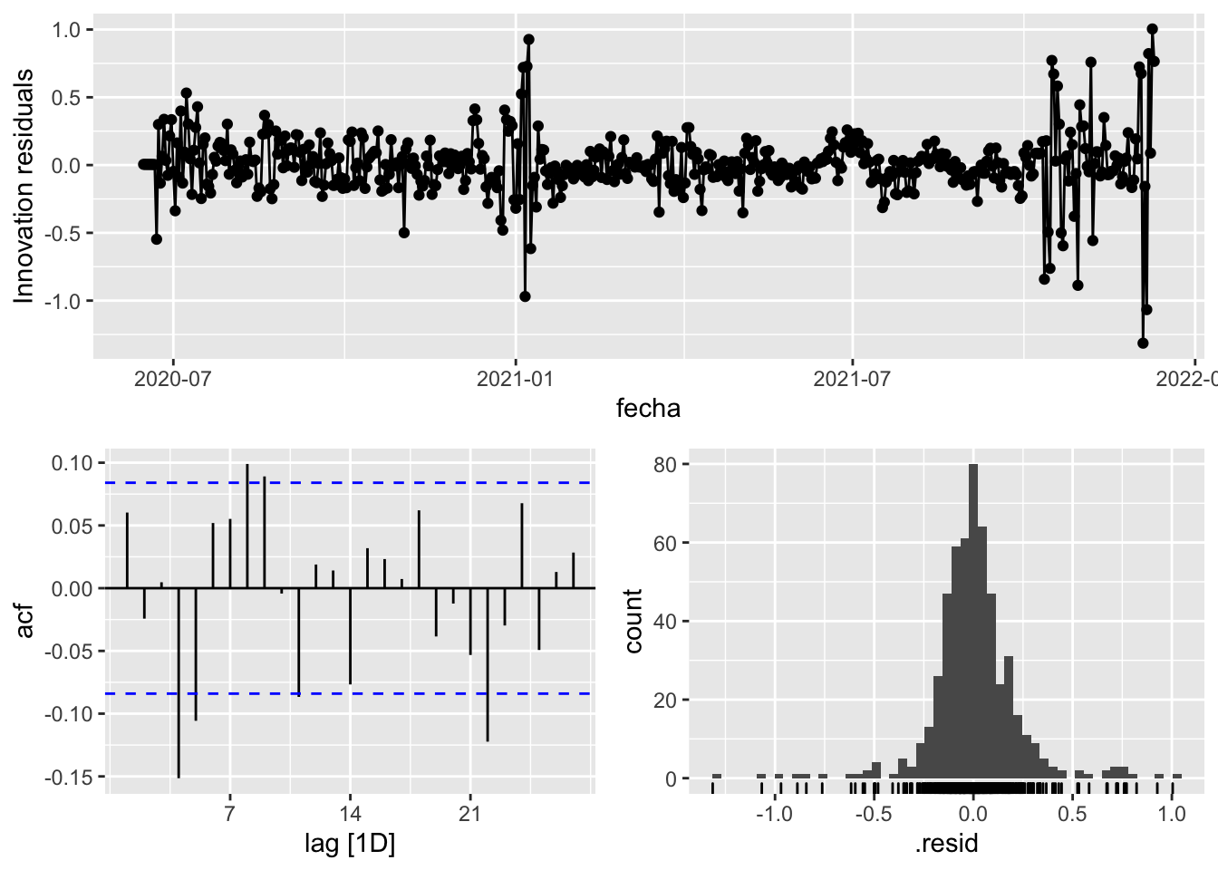
augment(fit_model) %>%
features(.innov, ljung_box, lag=7)# A tibble: 3 × 4
provincia .model lb_stat lb_pvalue
<chr> <chr> <dbl> <dbl>
1 Madrid arima_at1 15.6 0.0293
2 Madrid arima_at2 24.3 0.00102
3 Madrid Snaive 1470. 0 augment(fit_model) %>%
features(.innov, ljung_box, lag=14)# A tibble: 3 × 4
provincia .model lb_stat lb_pvalue
<chr> <chr> <dbl> <dbl>
1 Madrid arima_at1 46.6 0.0000224
2 Madrid arima_at2 41.9 0.000128
3 Madrid Snaive 2317. 0 augment(fit_model) %>%
features(.innov, ljung_box, lag=21)# A tibble: 3 × 4
provincia .model lb_stat lb_pvalue
<chr> <chr> <dbl> <dbl>
1 Madrid arima_at1 55.2 0.0000657
2 Madrid arima_at2 47.5 0.000801
3 Madrid Snaive 2574. 0 augment(fit_model) %>%
features(.innov, ljung_box, lag=57)# A tibble: 3 × 4
provincia .model lb_stat lb_pvalue
<chr> <chr> <dbl> <dbl>
1 Madrid arima_at1 124. 0.000000809
2 Madrid arima_at2 132. 0.0000000650
3 Madrid Snaive 3050. 0 # To predict future values of infections, we need to pass the model future/prediction values of the complementary variables tmed and mobility
# We are going to select those from the test dataset
data_fc_h7 <- data_Madrid_test %>%
select(-num_casos) %>%
slice(1:7)
data_fc_h14 <- data_Madrid_test %>%
select(-num_casos) %>%
slice(1:14)
data_fc_h21 <- data_Madrid_test %>%
select(-num_casos) %>%
slice(1:21)
data_fc_h57 <- data_Madrid_test %>%
select(-num_casos) %>%
slice(1:57)# Significant spikes out of 30 is still consistent with white noise
# To be sure, use a Ljung-Box test, which has a large p-value, confirming that
# the residuals are similar to white noise.
# Note that the alternative models also passed this test.
#
# Forecast
fc_h7 <- fabletools::forecast(fit_model, new_data = data_fc_h7)
fc_h14 <- fabletools::forecast(fit_model, new_data = data_fc_h14)
fc_h21 <- fabletools::forecast(fit_model, new_data = data_fc_h21)
fc_h57 <- fabletools::forecast(fit_model, new_data = data_fc_h57)7 days
# Plots
fc_h7 %>%
autoplot(
data_Madrid_test %>%
filter(fecha <= as.Date("2021-12-10", format = "%Y-%m-%d")+days(7))
) +
labs(y = "Nº cases", title = "Madrid - forecast h7")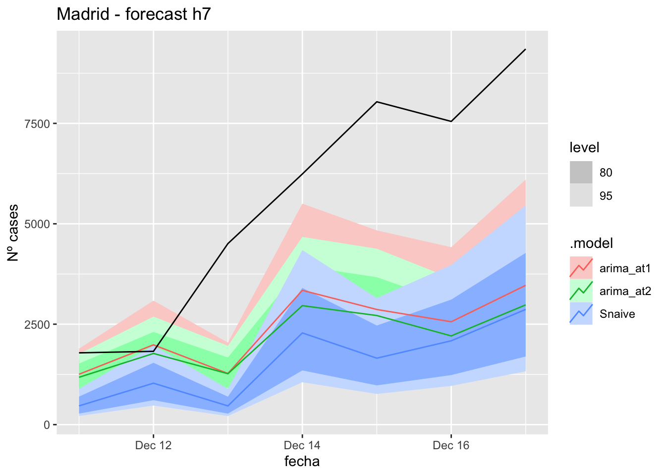
fc_h7 %>%
autoplot(
data_Madrid %>%
filter(fecha <= as.Date("2021-12-10", format = "%Y-%m-%d")+days(7) &
fecha > as.Date("2021-10-01", format = "%Y-%m-%d"))
) +
labs(y = "Nº cases", title = "Madrid - forecast h7")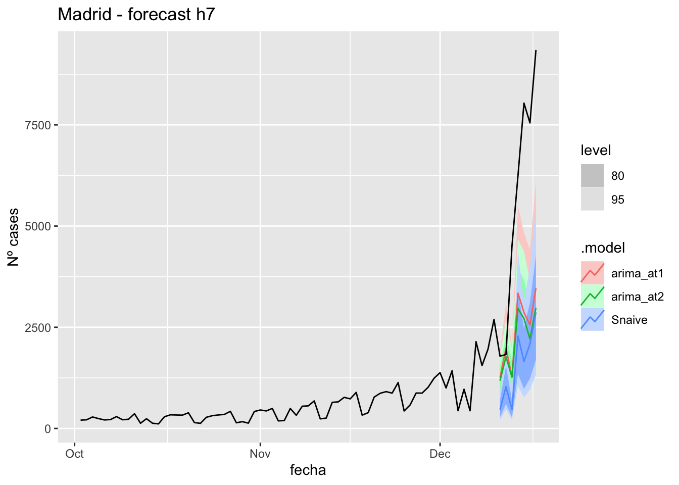
# Accuracy
fabletools::accuracy(fc_h7, data_Madrid)# A tibble: 3 × 11
.model provincia .type ME RMSE MAE MPE MAPE MASE RMSSE ACF1
<chr> <chr> <chr> <dbl> <dbl> <dbl> <dbl> <dbl> <dbl> <dbl> <dbl>
1 arima_at1 Madrid Test 3221. 3881. 3267. 47.5 50.0 8.15 6.03 0.505
2 arima_at2 Madrid Test 3459. 4124. 3459. 52.3 52.3 8.63 6.40 0.542
3 Snaive Madrid Test 4063. 4582. 4063. 70.2 70.2 10.1 7.12 0.49114 days
# Plots
fc_h14 %>%
autoplot(
data_Madrid_test %>%
filter(fecha <= as.Date("2021-12-10", format = "%Y-%m-%d")+days(14))
) +
labs(y = "Nº cases", title = "Madrid - forecast h14")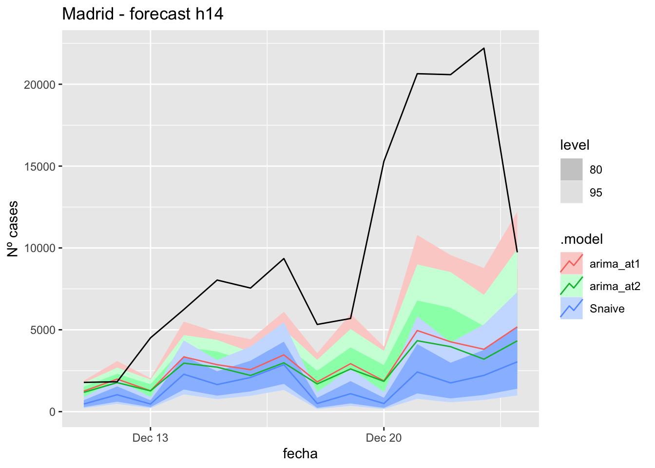
fc_h14 %>%
autoplot(
data_Madrid %>%
filter(fecha <= as.Date("2021-12-10", format = "%Y-%m-%d")+days(14) &
fecha > as.Date("2021-10-01", format = "%Y-%m-%d"))
) +
labs(y = "Nº cases", title = "Madrid - forecast h14")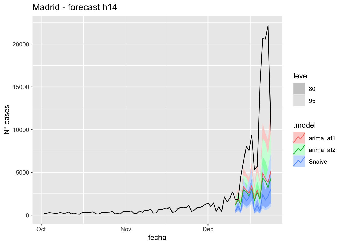
# Accuracy
fabletools::accuracy(fc_h14, data_Madrid)# A tibble: 3 × 11
.model provincia .type ME RMSE MAE MPE MAPE MASE RMSSE ACF1
<chr> <chr> <chr> <dbl> <dbl> <dbl> <dbl> <dbl> <dbl> <dbl> <dbl>
1 arima_at1 Madrid Test 6943. 9169. 6966. 58.5 59.8 17.4 14.2 0.616
2 arima_at2 Madrid Test 7265. 9468. 7265. 62.7 62.7 18.1 14.7 0.634
3 Snaive Madrid Test 8314. 10493. 8314. 78.4 78.4 20.7 16.3 0.68021 days
# Plots
fc_h21 %>%
autoplot(
data_Madrid_test %>%
filter(fecha <= as.Date("2021-12-10", format = "%Y-%m-%d")+days(21))
) +
labs(y = "Nº cases", title = "Madrid - forecast h21")
fc_h21 %>%
autoplot(
data_Madrid %>%
filter(fecha <= as.Date("2021-12-10", format = "%Y-%m-%d")+days(21) &
fecha > as.Date("2021-10-01", format = "%Y-%m-%d"))
) +
labs(y = "Nº cases", title = "Madrid - forecast h21")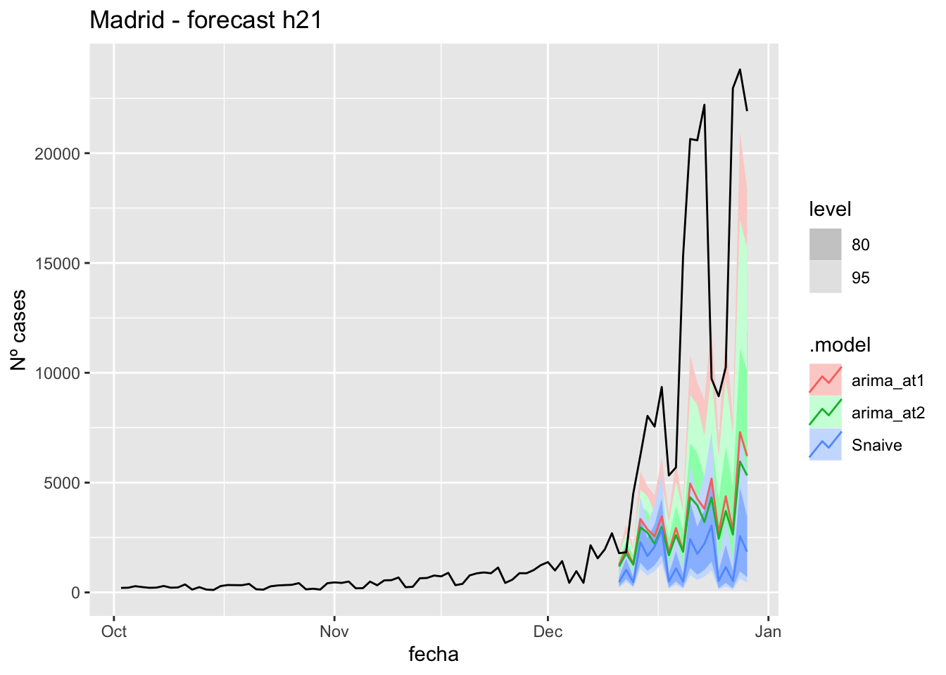
# Accuracy
fabletools::accuracy(fc_h21, data_Madrid)# A tibble: 3 × 11
.model provincia .type ME RMSE MAE MPE MAPE MASE RMSSE ACF1
<chr> <chr> <chr> <dbl> <dbl> <dbl> <dbl> <dbl> <dbl> <dbl> <dbl>
1 arima_at1 Madrid Test 8508. 10700. 8525. 61.9 62.8 21.3 16.6 0.578
2 arima_at2 Madrid Test 8921. 11114. 8921. 66.0 66.0 22.3 17.3 0.607
3 Snaive Madrid Test 10402. 12674. 10402. 82.1 82.1 25.9 19.7 0.66157 days
# Plots
fc_h57 %>%
autoplot(
data_Madrid_test %>%
filter(fecha <= as.Date("2021-12-10", format = "%Y-%m-%d")+days(57))
) +
labs(y = "Nº cases", title = "Madrid - forecast h57")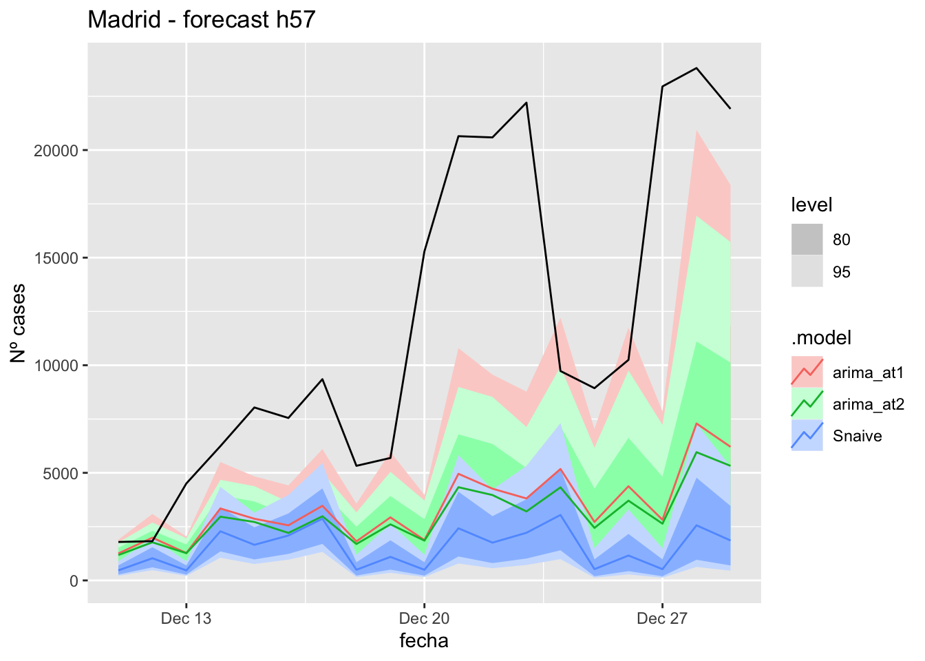
fc_h57 %>%
autoplot(
data_Madrid %>%
filter(fecha <= as.Date("2021-12-10", format = "%Y-%m-%d")+days(57) &
fecha > as.Date("2021-10-01", format = "%Y-%m-%d"))
) +
labs(y = "Nº cases", title = "Madrid - forecast h57")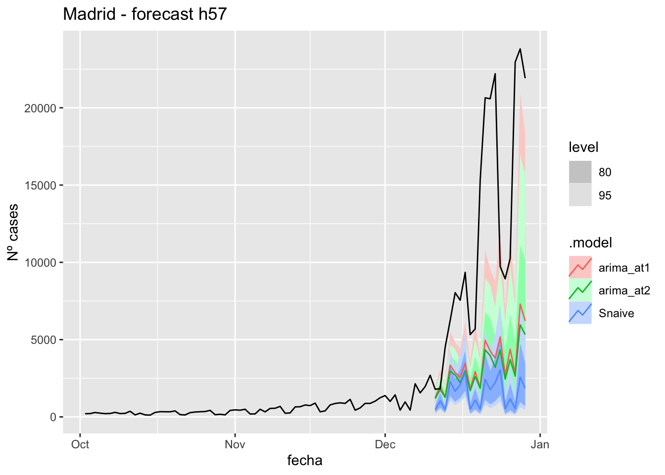
# Accuracy
fabletools::accuracy(fc_h57, data_Madrid)# A tibble: 3 × 11
.model provincia .type ME RMSE MAE MPE MAPE MASE RMSSE ACF1
<chr> <chr> <chr> <dbl> <dbl> <dbl> <dbl> <dbl> <dbl> <dbl> <dbl>
1 arima_at1 Madrid Test 8508. 10700. 8525. 61.9 62.8 21.3 16.6 0.578
2 arima_at2 Madrid Test 8921. 11114. 8921. 66.0 66.0 22.3 17.3 0.607
3 Snaive Madrid Test 10402. 12674. 10402. 82.1 82.1 25.9 19.7 0.661Malaga
data_Malaga <- covid_data %>%
filter(provincia == "Málaga") %>%
filter(fecha > as.Date("2020-06-14", format = "%Y-%m-%d")) %>%
select(provincia, fecha, num_casos, tmed, mob_flujo) %>%
drop_na() %>%
as_tsibble(key = provincia, index = fecha)
data_Malaga# A tsibble: 563 x 5 [1D]
# Key: provincia [1]
provincia fecha num_casos tmed mob_flujo
<chr> <date> <dbl> <dbl> <dbl>
1 Málaga 2020-06-15 1 27.2 18.9
2 Málaga 2020-06-16 1 27.8 19.8
3 Málaga 2020-06-17 2 26.9 19.9
4 Málaga 2020-06-18 2 21.6 20.0
5 Málaga 2020-06-19 1 24.7 20.1
6 Málaga 2020-06-20 4 22.6 18.1
7 Málaga 2020-06-21 4 22.7 18.8
8 Málaga 2020-06-22 6 25 19.5
9 Málaga 2020-06-23 8 25.6 20.2
10 Málaga 2020-06-24 65 24.5 21.0
# … with 553 more rowsdata_Malaga_train <- data_Malaga %>%
filter(fecha <= as.Date("2021-12-10", format = "%Y-%m-%d"))
summary(data_Malaga_train$fecha) Min. 1st Qu. Median Mean 3rd Qu. Max.
"2020-06-15" "2020-10-28" "2021-03-13" "2021-03-13" "2021-07-27" "2021-12-10" data_Malaga_test <- data_Malaga %>%
filter(fecha > as.Date("2021-12-10", format = "%Y-%m-%d"))
summary(data_Malaga_test$fecha) Min. 1st Qu. Median Mean 3rd Qu. Max.
"2021-12-11" "2021-12-15" "2021-12-20" "2021-12-20" "2021-12-24" "2021-12-29" # Lamba for num_casos
lambda_Malaga_casos <- data_Malaga %>%
features(num_casos, features = guerrero) %>%
pull(lambda_guerrero)
lambda_Malaga_casos[1] 0.2360418# Lamba for average temp
lambda_Malaga_tmed <- data_Malaga %>%
features(tmed, features = guerrero) %>%
pull(lambda_guerrero)
lambda_Malaga_tmed[1] 0.6474133# Lamba for mobility
lambda_Malaga_mobil <- data_Malaga %>%
features(mob_flujo, features = guerrero) %>%
pull(lambda_guerrero)
lambda_Malaga_mobil[1] 1.999927fit_model <- data_Malaga_train %>%
model(
arima_at1 = ARIMA(box_cox(num_casos, lambda_Malaga_casos) ~
box_cox(tmed, lambda_Malaga_tmed) +
box_cox(mob_flujo, lambda_Malaga_mobil)),
arima_at2 = ARIMA(box_cox(num_casos, lambda_Malaga_casos) ~
box_cox(tmed, lambda_Malaga_tmed) +
box_cox(mob_flujo, lambda_Malaga_mobil),
stepwise = FALSE, approx = FALSE),
Snaive = SNAIVE(box_cox(num_casos, lambda_Malaga_casos))
)
# Show and report model
fit_model# A mable: 1 x 4
# Key: provincia [1]
provincia arima_at1
<chr> <model>
1 Málaga <LM w/ ARIMA(2,0,3)(0,1,1)[7] errors>
# … with 2 more variables: arima_at2 <model>, Snaive <model>glance(fit_model)# A tibble: 3 × 9
provincia .model sigma2 log_lik AIC AICc BIC ar_roots ma_roots
<chr> <chr> <dbl> <dbl> <dbl> <dbl> <dbl> <list> <list>
1 Málaga arima_at1 0.550 -602. 1221. 1221. 1260. <cpl [2]> <cpl [10]>
2 Málaga arima_at2 0.550 -602. 1221. 1221. 1260. <cpl [2]> <cpl [10]>
3 Málaga Snaive 2.19 NA NA NA NA <NULL> <NULL> fit_model %>%
pivot_longer(-provincia,
names_to = ".model",
values_to = "orders") %>%
left_join(glance(fit_model), by = c("provincia", ".model")) %>%
arrange(AICc) %>%
select(.model:BIC)# A mable: 3 x 7
# Key: .model [3]
.model orders sigma2 log_lik AIC AICc BIC
<chr> <model> <dbl> <dbl> <dbl> <dbl> <dbl>
1 arima_… <LM w/ ARIMA(2,0,3)(0,1,1)[7] errors> 0.550 -602. 1221. 1221. 1260.
2 arima_… <LM w/ ARIMA(2,0,3)(0,1,1)[7] errors> 0.550 -602. 1221. 1221. 1260.
3 Snaive <SNAIVE> 2.19 NA NA NA NA # We use a Ljung-Box test >> large p-value, confirms residuals are similar / considered to white noise
fit_model %>%
select(Snaive) %>%
gg_tsresiduals()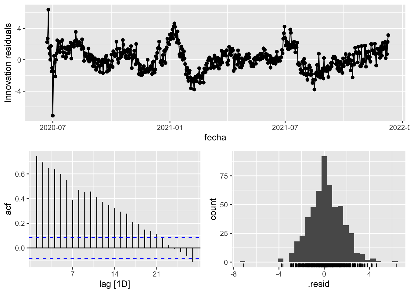
fit_model %>%
select(arima_at1) %>%
gg_tsresiduals()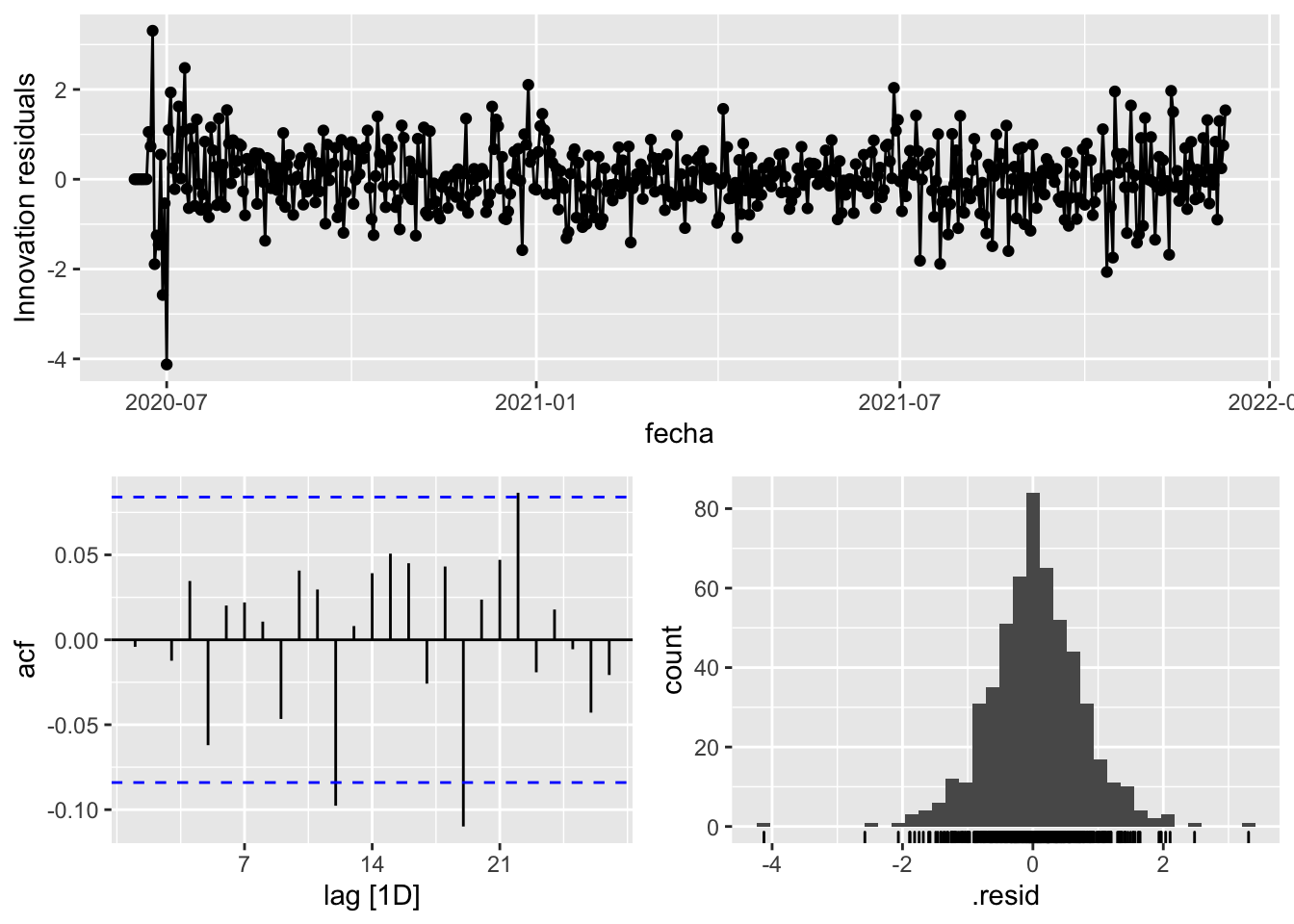
fit_model %>%
select(arima_at2) %>%
gg_tsresiduals()
augment(fit_model) %>%
features(.innov, ljung_box, lag=7)# A tibble: 3 × 4
provincia .model lb_stat lb_pvalue
<chr> <chr> <dbl> <dbl>
1 Málaga arima_at1 3.36 0.849
2 Málaga arima_at2 3.36 0.849
3 Málaga Snaive 1450. 0 augment(fit_model) %>%
features(.innov, ljung_box, lag=14)# A tibble: 3 × 4
provincia .model lb_stat lb_pvalue
<chr> <chr> <dbl> <dbl>
1 Málaga arima_at1 12.3 0.585
2 Málaga arima_at2 12.3 0.585
3 Málaga Snaive 2094. 0 augment(fit_model) %>%
features(.innov, ljung_box, lag=21)# A tibble: 3 × 4
provincia .model lb_stat lb_pvalue
<chr> <chr> <dbl> <dbl>
1 Málaga arima_at1 24.7 0.261
2 Málaga arima_at2 24.7 0.261
3 Málaga Snaive 2261. 0 augment(fit_model) %>%
features(.innov, ljung_box, lag=57)# A tibble: 3 × 4
provincia .model lb_stat lb_pvalue
<chr> <chr> <dbl> <dbl>
1 Málaga arima_at1 55.8 0.520
2 Málaga arima_at2 55.8 0.520
3 Málaga Snaive 3148. 0 # To predict future values of infections, we need to pass the model future/prediction values of the complementary variables tmed and mobility
# We are going to select those from the test dataset
data_fc_h7 <- data_Malaga_test %>%
select(-num_casos) %>%
slice(1:7)
data_fc_h14 <- data_Malaga_test %>%
select(-num_casos) %>%
slice(1:14)
data_fc_h21 <- data_Malaga_test %>%
select(-num_casos) %>%
slice(1:21)
data_fc_h57 <- data_Malaga_test %>%
select(-num_casos) %>%
slice(1:57)# Significant spikes out of 30 is still consistent with white noise
# To be sure, use a Ljung-Box test, which has a large p-value, confirming that
# the residuals are similar to white noise.
# Note that the alternative models also passed this test.
#
# Forecast
fc_h7 <- fabletools::forecast(fit_model, new_data = data_fc_h7)
fc_h14 <- fabletools::forecast(fit_model, new_data = data_fc_h14)
fc_h21 <- fabletools::forecast(fit_model, new_data = data_fc_h21)
fc_h57 <- fabletools::forecast(fit_model, new_data = data_fc_h57)7 days
# Plots
fc_h7 %>%
autoplot(
data_Malaga_test %>%
filter(fecha <= as.Date("2021-12-10", format = "%Y-%m-%d")+days(7))
) +
labs(y = "Nº cases", title = "Malaga - forecast h7")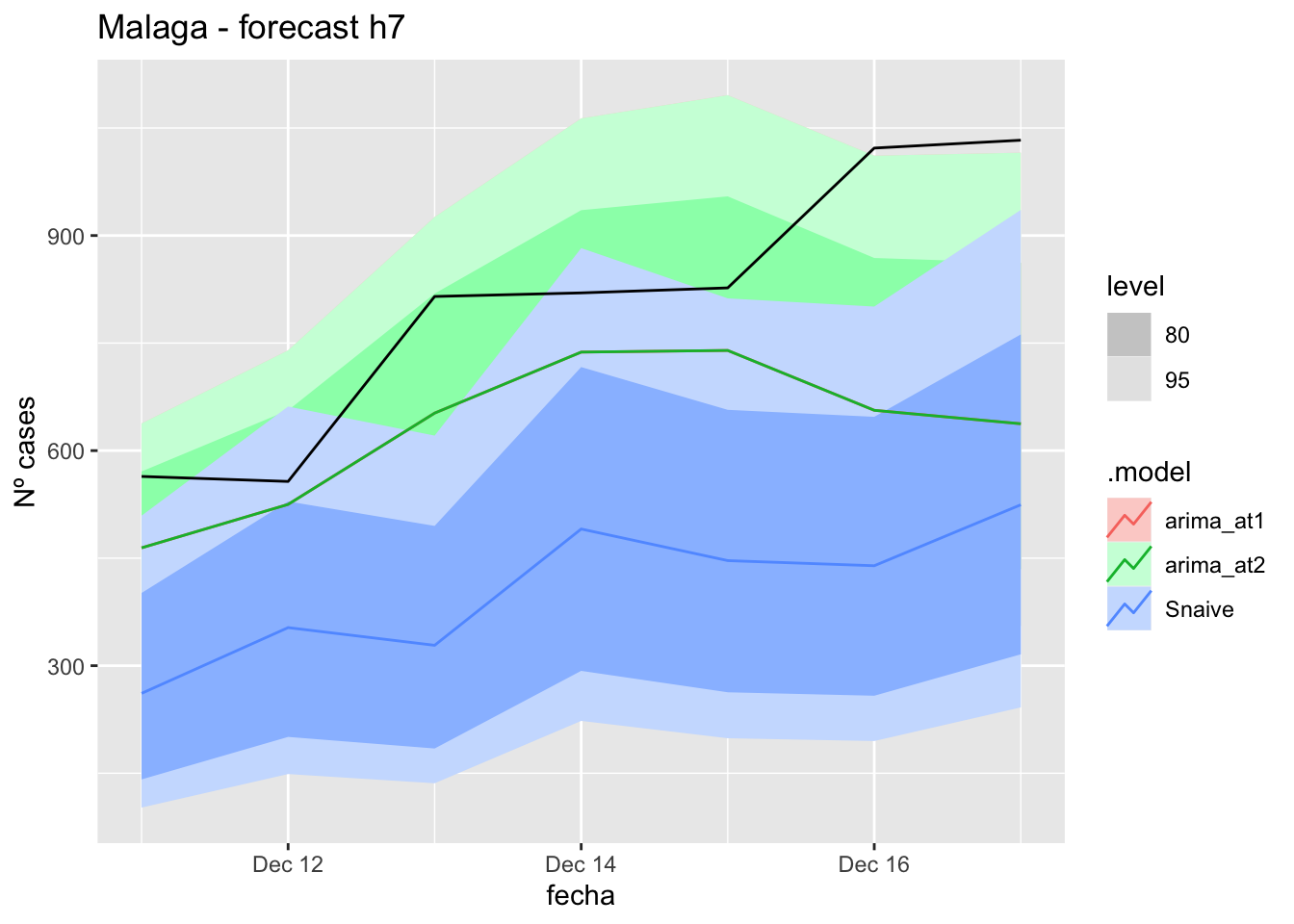
fc_h7 %>%
autoplot(
data_Malaga %>%
filter(fecha <= as.Date("2021-12-10", format = "%Y-%m-%d")+days(7) &
fecha > as.Date("2021-10-01", format = "%Y-%m-%d"))
) +
labs(y = "Nº cases", title = "Malaga - forecast h7")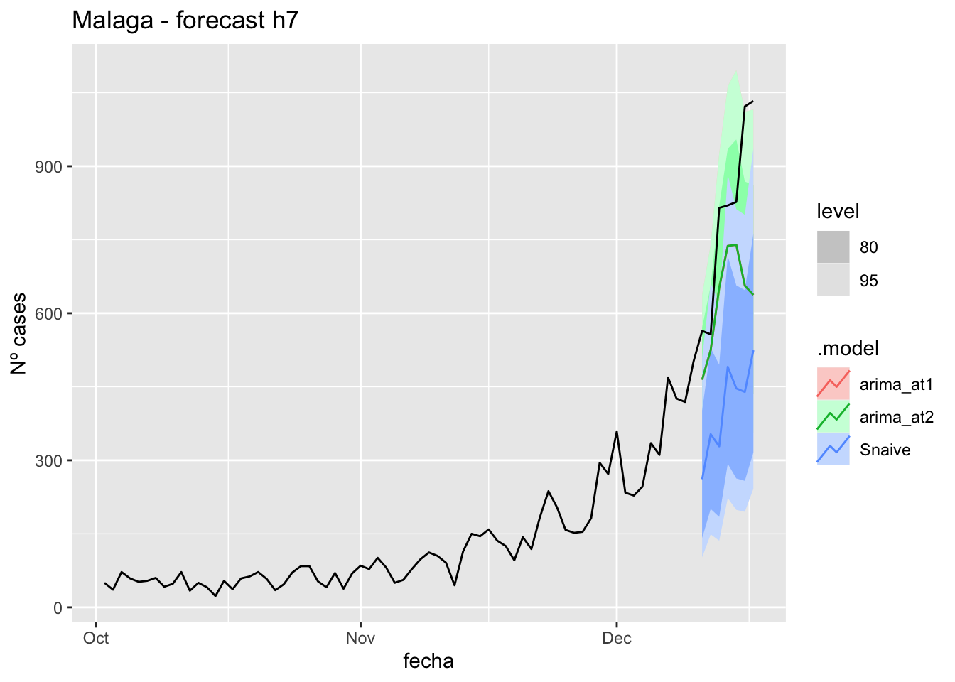
# Accuracy
fabletools::accuracy(fc_h7, data_Malaga)# A tibble: 3 × 11
.model provincia .type ME RMSE MAE MPE MAPE MASE RMSSE ACF1
<chr> <chr> <chr> <dbl> <dbl> <dbl> <dbl> <dbl> <dbl> <dbl> <dbl>
1 arima_at1 Málaga Test 175. 221. 175. 19.7 19.7 1.88 1.37 0.370
2 arima_at2 Málaga Test 175. 221. 175. 19.7 19.7 1.88 1.37 0.370
3 Snaive Málaga Test 399. 418. 399. 48.9 48.9 4.29 2.58 0.12914 days
# Plots
fc_h14 %>%
autoplot(
data_Malaga_test %>%
filter(fecha <= as.Date("2021-12-10", format = "%Y-%m-%d")+days(14))
) +
labs(y = "Nº cases", title = "Malaga - forecast h14")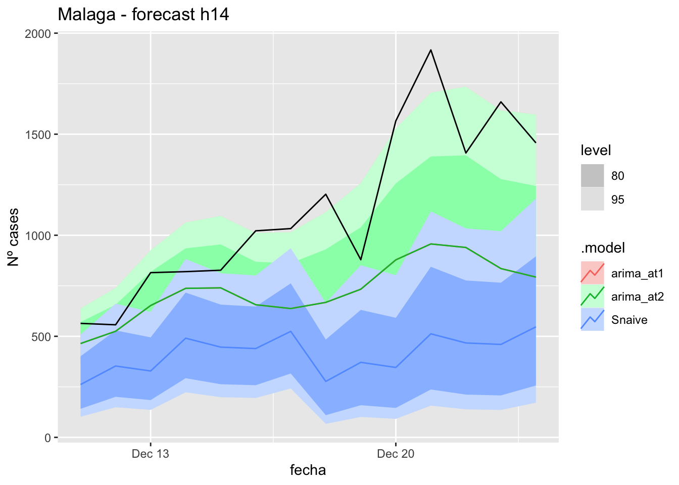
fc_h14 %>%
autoplot(
data_Malaga %>%
filter(fecha <= as.Date("2021-12-10", format = "%Y-%m-%d")+days(14) &
fecha > as.Date("2021-10-01", format = "%Y-%m-%d"))
) +
labs(y = "Nº cases", title = "Malaga - forecast h14")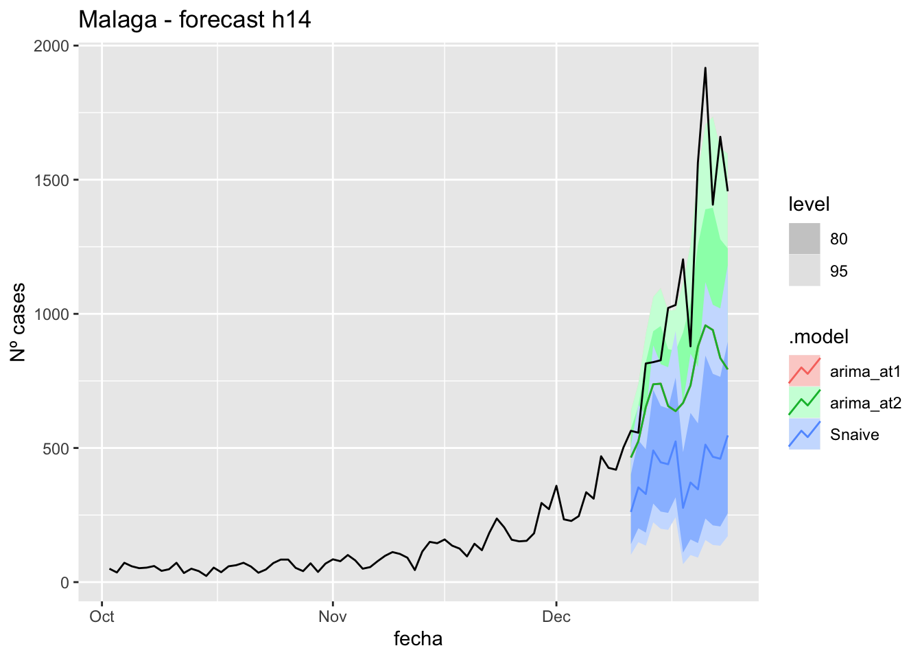
# Accuracy
fabletools::accuracy(fc_h14, data_Malaga)# A tibble: 3 × 11
.model provincia .type ME RMSE MAE MPE MAPE MASE RMSSE ACF1
<chr> <chr> <chr> <dbl> <dbl> <dbl> <dbl> <dbl> <dbl> <dbl> <dbl>
1 arima_at1 Málaga Test 394. 492. 394. 30.1 30.1 4.23 3.04 0.506
2 arima_at2 Málaga Test 394. 492. 394. 30.1 30.1 4.23 3.04 0.506
3 Snaive Málaga Test 707. 800. 707. 59.3 59.3 7.60 4.94 0.58221 days
# Plots
fc_h21 %>%
autoplot(
data_Malaga_test %>%
filter(fecha <= as.Date("2021-12-10", format = "%Y-%m-%d")+days(21))
) +
labs(y = "Nº cases", title = "Malaga - forecast h21")
fc_h21 %>%
autoplot(
data_Malaga %>%
filter(fecha <= as.Date("2021-12-10", format = "%Y-%m-%d")+days(21) &
fecha > as.Date("2021-10-01", format = "%Y-%m-%d"))
) +
labs(y = "Nº cases", title = "Malaga - forecast h21")
# Accuracy
fabletools::accuracy(fc_h21, data_Malaga)# A tibble: 3 × 11
.model provincia .type ME RMSE MAE MPE MAPE MASE RMSSE ACF1
<chr> <chr> <chr> <dbl> <dbl> <dbl> <dbl> <dbl> <dbl> <dbl> <dbl>
1 arima_at1 Málaga Test 588. 785. 588. 35.4 35.4 6.32 4.85 0.529
2 arima_at2 Málaga Test 588. 785. 588. 35.4 35.4 6.32 4.85 0.529
3 Snaive Málaga Test 964. 1149. 964. 64.5 64.5 10.4 7.10 0.59057 days
# Plots
fc_h57 %>%
autoplot(
data_Malaga_test %>%
filter(fecha <= as.Date("2021-12-10", format = "%Y-%m-%d")+days(57))
) +
labs(y = "Nº cases", title = "Malaga - forecast h57")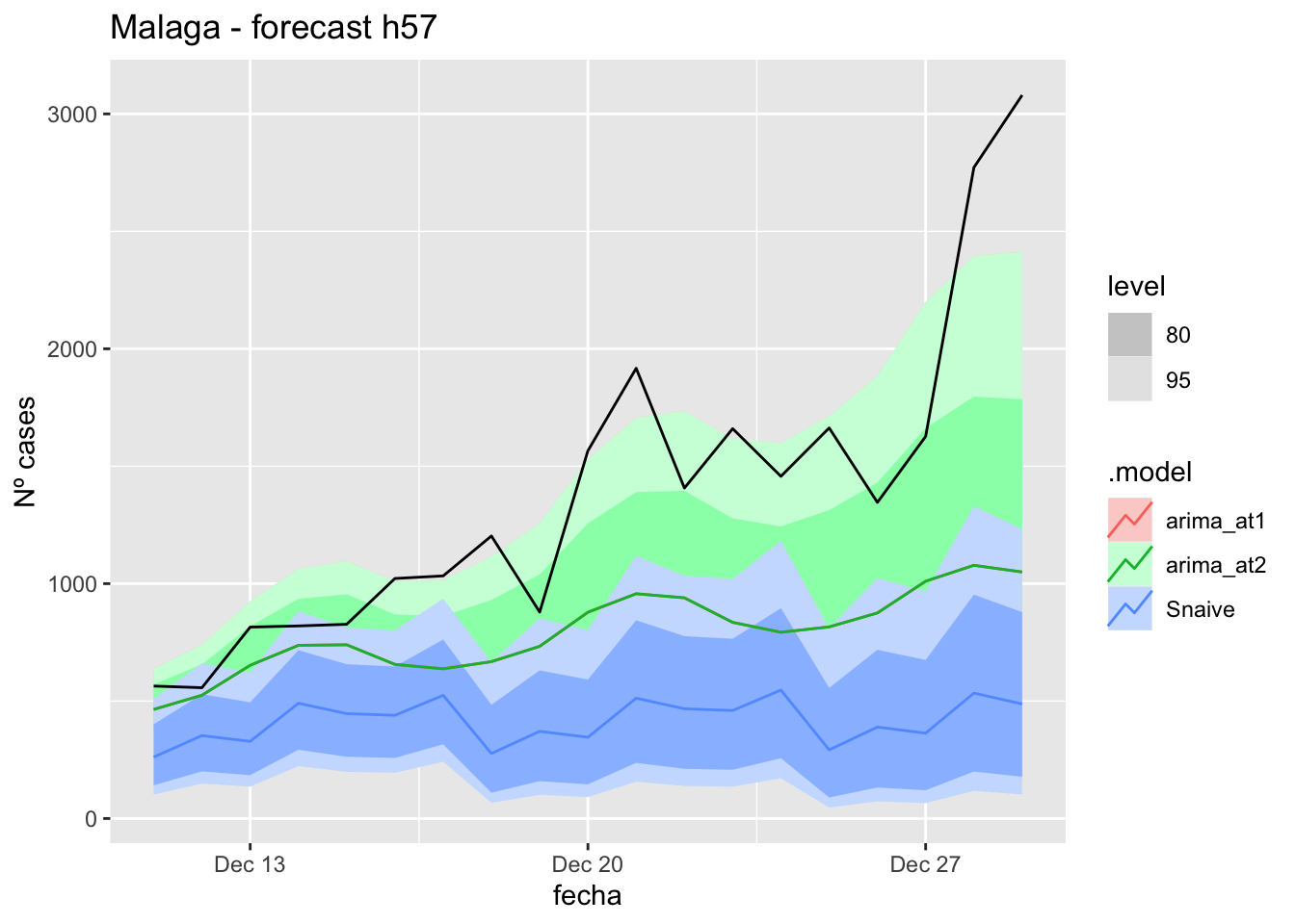
fc_h57 %>%
autoplot(
data_Malaga %>%
filter(fecha <= as.Date("2021-12-10", format = "%Y-%m-%d")+days(57) &
fecha > as.Date("2021-10-01", format = "%Y-%m-%d"))
) +
labs(y = "Nº cases", title = "Malaga - forecast h57")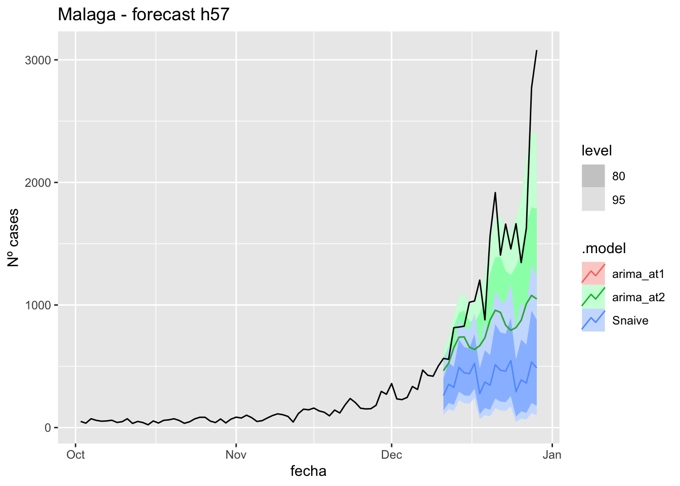
# Accuracy
fabletools::accuracy(fc_h57, data_Malaga)# A tibble: 3 × 11
.model provincia .type ME RMSE MAE MPE MAPE MASE RMSSE ACF1
<chr> <chr> <chr> <dbl> <dbl> <dbl> <dbl> <dbl> <dbl> <dbl> <dbl>
1 arima_at1 Málaga Test 588. 785. 588. 35.4 35.4 6.32 4.85 0.529
2 arima_at2 Málaga Test 588. 785. 588. 35.4 35.4 6.32 4.85 0.529
3 Snaive Málaga Test 964. 1149. 964. 64.5 64.5 10.4 7.10 0.590Sevilla
data_Sevilla <- covid_data %>%
filter(provincia == "Sevilla") %>%
filter(fecha > as.Date("2020-06-14", format = "%Y-%m-%d")) %>%
select(provincia, fecha, num_casos, tmed, mob_flujo) %>%
drop_na() %>%
as_tsibble(key = provincia, index = fecha)
data_Sevilla# A tsibble: 563 x 5 [1D]
# Key: provincia [1]
provincia fecha num_casos tmed mob_flujo
<chr> <date> <dbl> <dbl> <dbl>
1 Sevilla 2020-06-15 2 23.1 19.9
2 Sevilla 2020-06-16 1 24.0 20.8
3 Sevilla 2020-06-17 0 24.9 21.1
4 Sevilla 2020-06-18 0 25.8 21.3
5 Sevilla 2020-06-19 0 26.6 21.2
6 Sevilla 2020-06-20 0 27.5 18.0
7 Sevilla 2020-06-21 0 28.4 18.9
8 Sevilla 2020-06-22 1 29.3 19.8
9 Sevilla 2020-06-23 0 30.2 20.7
10 Sevilla 2020-06-24 1 29.4 21.6
# … with 553 more rowsdata_Sevilla_train <- data_Sevilla %>%
filter(fecha <= as.Date("2021-12-10", format = "%Y-%m-%d"))
summary(data_Sevilla_train$fecha) Min. 1st Qu. Median Mean 3rd Qu. Max.
"2020-06-15" "2020-10-28" "2021-03-13" "2021-03-13" "2021-07-27" "2021-12-10" data_Sevilla_test <- data_Sevilla %>%
filter(fecha > as.Date("2021-12-10", format = "%Y-%m-%d"))
summary(data_Sevilla_test$fecha) Min. 1st Qu. Median Mean 3rd Qu. Max.
"2021-12-11" "2021-12-15" "2021-12-20" "2021-12-20" "2021-12-24" "2021-12-29" # Lamba for num_casos
lambda_Sevilla_casos <- data_Sevilla %>%
features(num_casos, features = guerrero) %>%
pull(lambda_guerrero)
lambda_Sevilla_casos[1] 0.2191951# Lamba for average temp
lambda_Sevilla_tmed <- data_Sevilla %>%
features(tmed, features = guerrero) %>%
pull(lambda_guerrero)
lambda_Sevilla_tmed[1] 1.057197# Lamba for mobility
lambda_Sevilla_mobil <- data_Sevilla %>%
features(mob_flujo, features = guerrero) %>%
pull(lambda_guerrero)
lambda_Sevilla_mobil[1] 0.7413917fit_model <- data_Sevilla_train %>%
model(
arima_at1 = ARIMA(box_cox(num_casos, lambda_Sevilla_casos) ~
box_cox(tmed, lambda_Sevilla_tmed) +
box_cox(mob_flujo, lambda_Sevilla_mobil)),
arima_at2 = ARIMA(box_cox(num_casos, lambda_Sevilla_casos) ~
box_cox(tmed, lambda_Sevilla_tmed) +
box_cox(mob_flujo, lambda_Sevilla_mobil),
stepwise = FALSE, approx = FALSE),
Snaive = SNAIVE(box_cox(num_casos, lambda_Sevilla_casos))
)
# Show and report model
fit_model# A mable: 1 x 4
# Key: provincia [1]
provincia arima_at1
<chr> <model>
1 Sevilla <LM w/ ARIMA(4,0,0)(2,1,0)[7] errors>
# … with 2 more variables: arima_at2 <model>, Snaive <model>glance(fit_model)# A tibble: 3 × 9
provincia .model sigma2 log_lik AIC AICc BIC ar_roots ma_roots
<chr> <chr> <dbl> <dbl> <dbl> <dbl> <dbl> <list> <list>
1 Sevilla arima_at1 0.917 -737. 1491. 1491. 1530. <cpl [18]> <cpl [0]>
2 Sevilla arima_at2 0.866 -722. 1462. 1463. 1501. <cpl [1]> <cpl [11]>
3 Sevilla Snaive 2.25 NA NA NA NA <NULL> <NULL> fit_model %>%
pivot_longer(-provincia,
names_to = ".model",
values_to = "orders") %>%
left_join(glance(fit_model), by = c("provincia", ".model")) %>%
arrange(AICc) %>%
select(.model:BIC)# A mable: 3 x 7
# Key: .model [3]
.model orders sigma2 log_lik AIC AICc BIC
<chr> <model> <dbl> <dbl> <dbl> <dbl> <dbl>
1 arima_… <LM w/ ARIMA(1,0,4)(0,1,1)[7] errors> 0.866 -722. 1462. 1463. 1501.
2 arima_… <LM w/ ARIMA(4,0,0)(2,1,0)[7] errors> 0.917 -737. 1491. 1491. 1530.
3 Snaive <SNAIVE> 2.25 NA NA NA NA # We use a Ljung-Box test >> large p-value, confirms residuals are similar / considered to white noise
fit_model %>%
select(Snaive) %>%
gg_tsresiduals()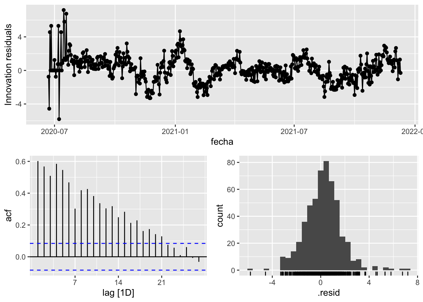
fit_model %>%
select(arima_at1) %>%
gg_tsresiduals()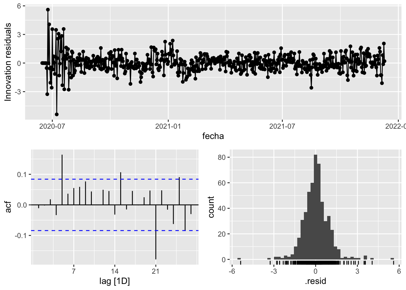
fit_model %>%
select(arima_at2) %>%
gg_tsresiduals()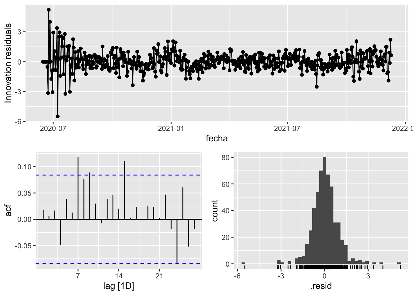
augment(fit_model) %>%
features(.innov, ljung_box, lag=7)# A tibble: 3 × 4
provincia .model lb_stat lb_pvalue
<chr> <chr> <dbl> <dbl>
1 Sevilla arima_at1 18.1 0.0113
2 Sevilla arima_at2 10.3 0.173
3 Sevilla Snaive 1028. 0 augment(fit_model) %>%
features(.innov, ljung_box, lag=14)# A tibble: 3 × 4
provincia .model lb_stat lb_pvalue
<chr> <chr> <dbl> <dbl>
1 Sevilla arima_at1 27.5 0.0167
2 Sevilla arima_at2 20.7 0.109
3 Sevilla Snaive 1507. 0 augment(fit_model) %>%
features(.innov, ljung_box, lag=21)# A tibble: 3 × 4
provincia .model lb_stat lb_pvalue
<chr> <chr> <dbl> <dbl>
1 Sevilla arima_at1 54.8 0.0000749
2 Sevilla arima_at2 28.5 0.126
3 Sevilla Snaive 1658. 0 augment(fit_model) %>%
features(.innov, ljung_box, lag=57)# A tibble: 3 × 4
provincia .model lb_stat lb_pvalue
<chr> <chr> <dbl> <dbl>
1 Sevilla arima_at1 115. 0.00000863
2 Sevilla arima_at2 77.8 0.0352
3 Sevilla Snaive 2098. 0 # To predict future values of infections, we need to pass the model future/prediction values of the complementary variables tmed and mobility
# We are going to select those from the test dataset
data_fc_h7 <- data_Sevilla_test %>%
select(-num_casos) %>%
slice(1:7)
data_fc_h14 <- data_Sevilla_test %>%
select(-num_casos) %>%
slice(1:14)
data_fc_h21 <- data_Sevilla_test %>%
select(-num_casos) %>%
slice(1:21)
data_fc_h57 <- data_Sevilla_test %>%
select(-num_casos) %>%
slice(1:57)# Significant spikes out of 30 is still consistent with white noise
# To be sure, use a Ljung-Box test, which has a large p-value, confirming that
# the residuals are similar to white noise.
# Note that the alternative models also passed this test.
#
# Forecast
fc_h7 <- fabletools::forecast(fit_model, new_data = data_fc_h7)
fc_h14 <- fabletools::forecast(fit_model, new_data = data_fc_h14)
fc_h21 <- fabletools::forecast(fit_model, new_data = data_fc_h21)
fc_h57 <- fabletools::forecast(fit_model, new_data = data_fc_h57)7 days
# Plots
fc_h7 %>%
autoplot(
data_Sevilla_test %>%
filter(fecha <= as.Date("2021-12-10", format = "%Y-%m-%d")+days(7))
) +
labs(y = "Nº cases", title = "Sevilla - forecast h7")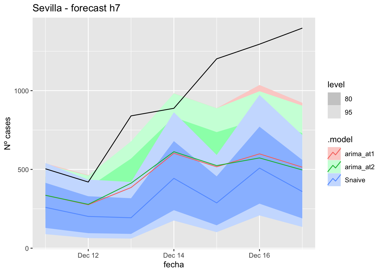
fc_h7 %>%
autoplot(
data_Sevilla %>%
filter(fecha <= as.Date("2021-12-10", format = "%Y-%m-%d")+days(7) &
fecha > as.Date("2021-10-01", format = "%Y-%m-%d"))
) +
labs(y = "Nº cases", title = "Sevilla - forecast h7")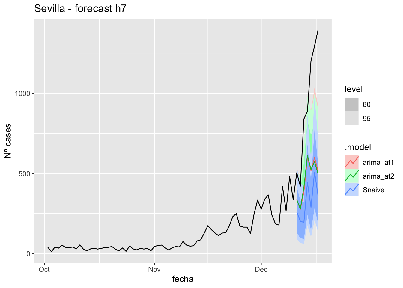
# Accuracy
fabletools::accuracy(fc_h7, data_Sevilla)# A tibble: 3 × 11
.model provincia .type ME RMSE MAE MPE MAPE MASE RMSSE ACF1
<chr> <chr> <chr> <dbl> <dbl> <dbl> <dbl> <dbl> <dbl> <dbl> <dbl>
1 arima_at1 Sevilla Test 474. 544. 474. 46.8 46.8 5.00 3.62 0.418
2 arima_at2 Sevilla Test 473. 548. 473. 46.5 46.5 4.99 3.64 0.457
3 Snaive Sevilla Test 613. 682. 613. 62.7 62.7 6.47 4.53 0.32414 days
# Plots
fc_h14 %>%
autoplot(
data_Sevilla_test %>%
filter(fecha <= as.Date("2021-12-10", format = "%Y-%m-%d")+days(14))
) +
labs(y = "Nº cases", title = "Sevilla - forecast h14")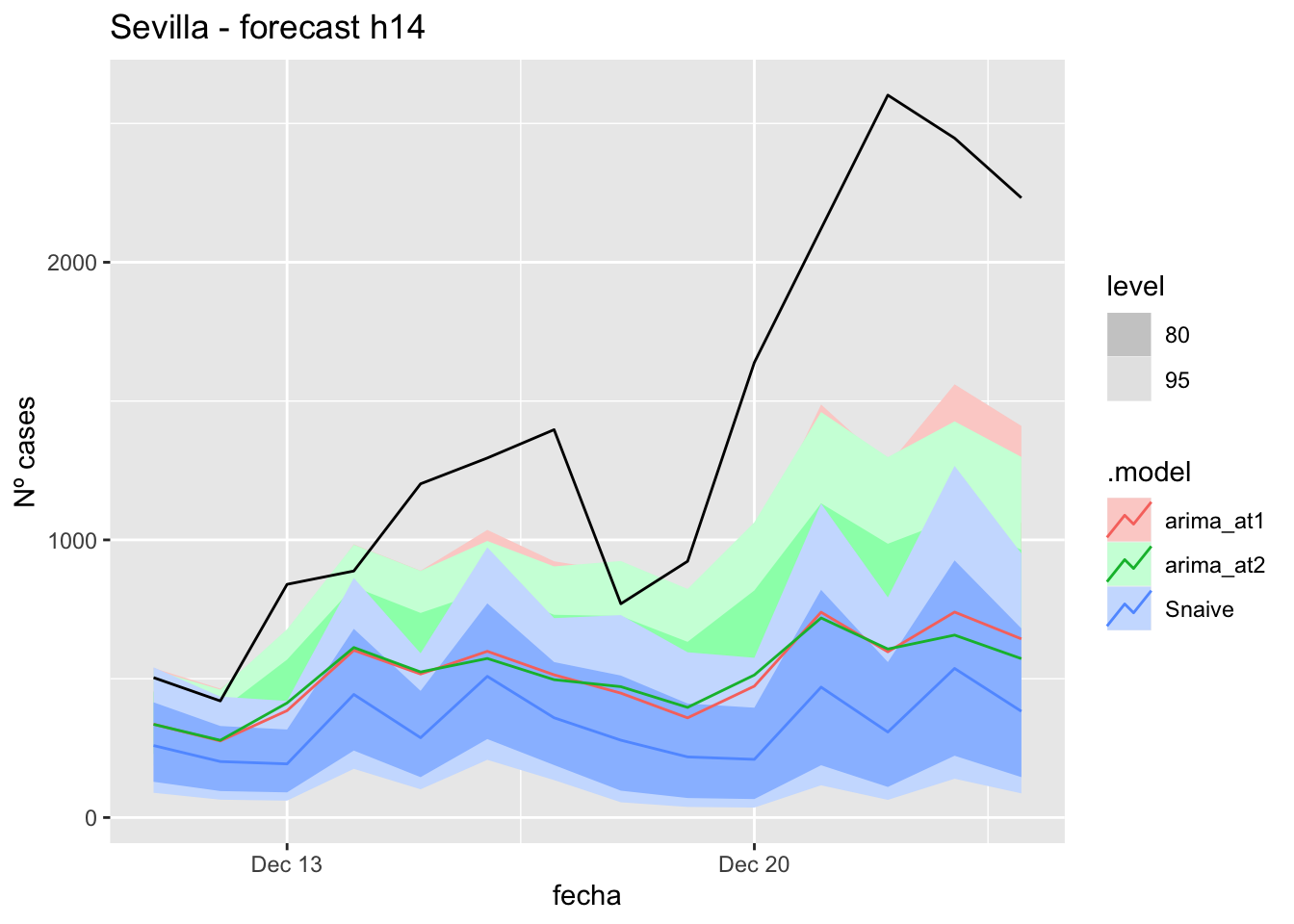
fc_h14 %>%
autoplot(
data_Sevilla %>%
filter(fecha <= as.Date("2021-12-10", format = "%Y-%m-%d")+days(14) &
fecha > as.Date("2021-12-10", format = "%Y-%m-%d"))
) +
labs(y = "Nº cases", title = "Sevilla - forecast h14")
# Accuracy
fabletools::accuracy(fc_h14, data_Sevilla)# A tibble: 3 × 11
.model provincia .type ME RMSE MAE MPE MAPE MASE RMSSE ACF1
<chr> <chr> <chr> <dbl> <dbl> <dbl> <dbl> <dbl> <dbl> <dbl> <dbl>
1 arima_at1 Sevilla Test 861. 1043. 861. 56.1 56.1 9.08 6.93 0.731
2 arima_at2 Sevilla Test 865. 1057. 865. 55.7 55.7 9.12 7.03 0.741
3 Snaive Sevilla Test 1045. 1227. 1045. 70.9 70.9 11.0 8.16 0.71721 days
# Plots
fc_h21 %>%
autoplot(
data_Sevilla_test %>%
filter(fecha <= as.Date("2021-12-10", format = "%Y-%m-%d")+days(21))
) +
labs(y = "Nº cases", title = "Sevilla - forecast h21")
fc_h21 %>%
autoplot(
data_Sevilla %>%
filter(fecha <= as.Date("2021-12-10", format = "%Y-%m-%d")+days(21) &
fecha > as.Date("2021-10-01", format = "%Y-%m-%d"))
) +
labs(y = "Nº cases", title = "Sevilla - forecast h21")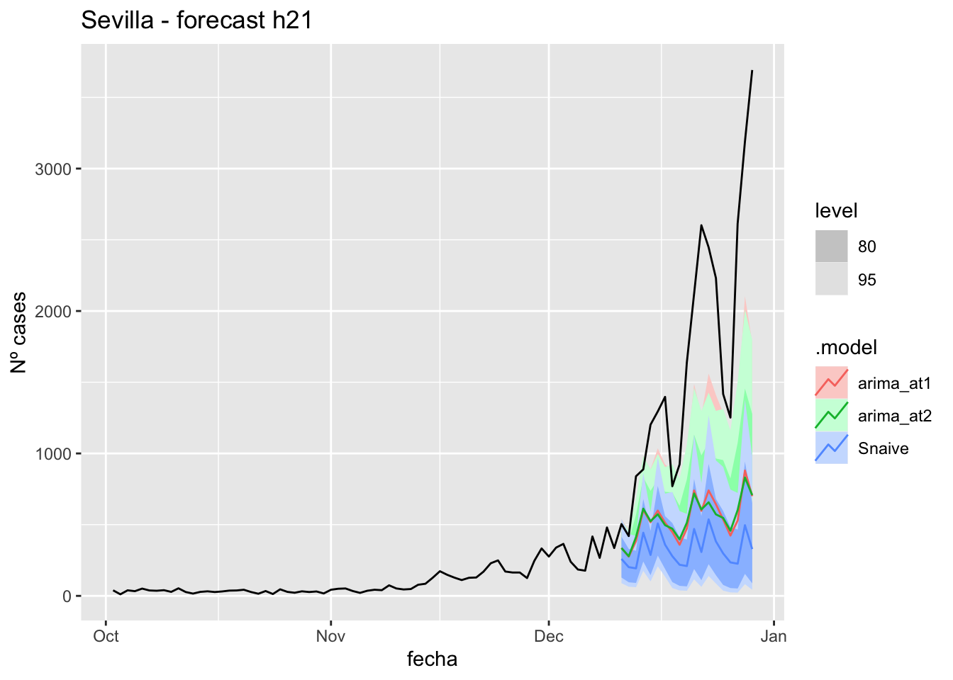
# Accuracy
fabletools::accuracy(fc_h21, data_Sevilla)# A tibble: 3 × 11
.model provincia .type ME RMSE MAE MPE MAPE MASE RMSSE ACF1
<chr> <chr> <chr> <dbl> <dbl> <dbl> <dbl> <dbl> <dbl> <dbl> <dbl>
1 arima_at1 Sevilla Test 1113. 1364. 1113. 60.3 60.3 11.7 9.07 0.634
2 arima_at2 Sevilla Test 1112. 1368. 1112. 59.8 59.8 11.7 9.10 0.644
3 Snaive Sevilla Test 1327. 1584. 1327. 74.7 74.7 14.0 10.5 0.63857 days
# Plots
fc_h57 %>%
autoplot(
data_Sevilla_test %>%
filter(fecha <= as.Date("2021-12-10", format = "%Y-%m-%d")+days(57))
) +
labs(y = "Nº cases", title = "Sevilla - forecast h57")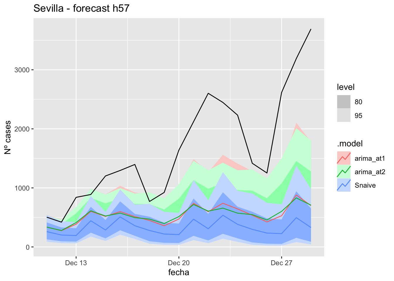
fc_h57 %>%
autoplot(
data_Sevilla %>%
filter(fecha <= as.Date("2021-12-10", format = "%Y-%m-%d")+days(57) &
fecha > as.Date("2021-10-01", format = "%Y-%m-%d"))
) +
labs(y = "Nº cases", title = "Sevilla - forecast h57")
# Accuracy
fabletools::accuracy(fc_h57, data_Sevilla)# A tibble: 3 × 11
.model provincia .type ME RMSE MAE MPE MAPE MASE RMSSE ACF1
<chr> <chr> <chr> <dbl> <dbl> <dbl> <dbl> <dbl> <dbl> <dbl> <dbl>
1 arima_at1 Sevilla Test 1113. 1364. 1113. 60.3 60.3 11.7 9.07 0.634
2 arima_at2 Sevilla Test 1112. 1368. 1112. 59.8 59.8 11.7 9.10 0.644
3 Snaive Sevilla Test 1327. 1584. 1327. 74.7 74.7 14.0 10.5 0.638