Task 3: Visual analysis

Introduction

As previously mentioned, the visual analysis will focus on the following provinces:

• Asturias
• Barcelona
• Madrid
• Málaga
• Sevilla

First, we need to load packages and clean data generated during previous tasks:

pacman::p_load(
      here,      # file locator
      tidyverse, # data management and ggplot2 graphics
      skimr,     # get overview of data
      janitor,   # produce and adorn tabulations and cross-tabulations
      lubridate, # manage dates
      PerformanceAnalytics,
      factoextra
)

covid_data <- readRDS(here("data", "clean", "final_covid_data.rds"))
covid_data

# A tibble: 4,095 × 26
   provincia fecha      num_casos num_casos_prueba_pcr num_casos_prueba_test_ac
   <chr>     <date>         <dbl>                <dbl>                    <dbl>
 1 Barcelona 2020-01-01         0                    0                        0
 2 Madrid    2020-01-01         1                    1                        0
 3 Málaga    2020-01-01         0                    0                        0
 4 Asturias  2020-01-01         0                    0                        0
 5 Sevilla   2020-01-01         0                    0                        0
 6 Barcelona 2020-01-02         0                    0                        0
 7 Madrid    2020-01-02         0                    0                        0
 8 Málaga    2020-01-02         0                    0                        0
 9 Asturias  2020-01-02         0                    0                        0
10 Sevilla   2020-01-02         0                    0                        0
# … with 4,085 more rows, and 21 more variables: num_casos_prueba_ag <dbl>,
#   num_casos_prueba_elisa <dbl>, num_casos_prueba_desconocida <dbl>,
#   num_hosp <dbl>, num_uci <dbl>, num_def <dbl>, tmed <dbl>, prec <dbl>,
#   tmin <dbl>, tmax <dbl>, wd <dbl>, ws <dbl>, ws_max <dbl>, sol <dbl>,
#   mob_grocery_pharmacy <dbl>, mob_parks <dbl>, mob_residential <dbl>,
#   mob_retail_recreation <dbl>, mob_transit_stations <dbl>,
#   mob_workplaces <dbl>, mob_flujo <dbl>

Covid-19 indicatives

Number of cases

According to CNE, in the evolution of the COVID-19 pandemic in Spain, there have been six periods:

• First period: From the beginning of the pandemic until June 21, 2020, date on which the state of alarm in Spain ended after the end of the first epidemic outbreak of COVID-19.

• Second period: June 22 through December 6, 2020, the turning point of the 14-day cumulative incidence (CI) of COVID-19 cases, between the second and third periods.

• Third period: December 7, 2020 through March 14, 2021, AI tipping point at 14 days of COVID-19 cases, between the third and fourth epidemic periods.

• Fourth period: March 15, 2021 through June 19, the 14-day AI tipping point for COVID-19 cases, between the fourth and fifth epidemic periods.

• Fifth period: June 20, 2021 through October 13, AI tipping point at 14 days of COVID-19 cases, between the fifth and sixth epidemic periods.

• Sixth period: From October 14, 2021 to the present, which may vary depending on the epidemiological situation of the pandemic in Spain.

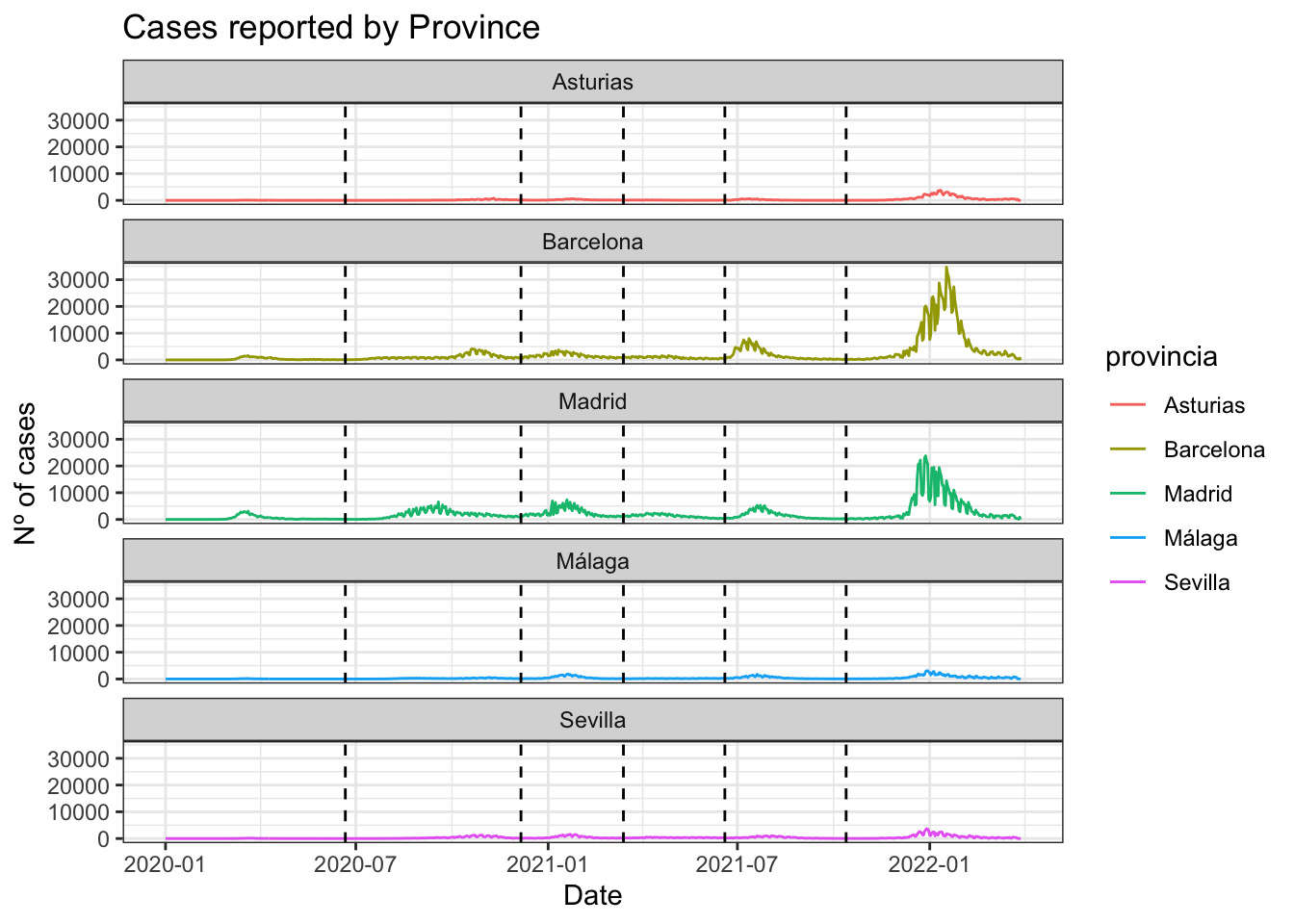
In the following plots, those periods are marked with vertical dashed lines.

covid_data %>% 
      ggplot(aes(x = fecha, y = num_casos)) +
      geom_line(aes(color = provincia)) +
      geom_vline(xintercept = as.Date("2020-06-21", format = "%Y-%m-%d"), linetype="dashed") +
      geom_vline(xintercept = as.Date("2020-12-06", format = "%Y-%m-%d"), linetype="dashed") +
      geom_vline(xintercept = as.Date("2021-03-14", format = "%Y-%m-%d"), linetype="dashed") +
      geom_vline(xintercept = as.Date("2021-06-19", format = "%Y-%m-%d"), linetype="dashed") +
      geom_vline(xintercept = as.Date("2021-10-13", format = "%Y-%m-%d"), linetype="dashed") +
      facet_wrap(~provincia, ncol=1) +
      theme(legend.position = "top") +
      labs(title="Cases reported by Province",
           x ="Date", y = "Nº of cases") +
      theme_bw()

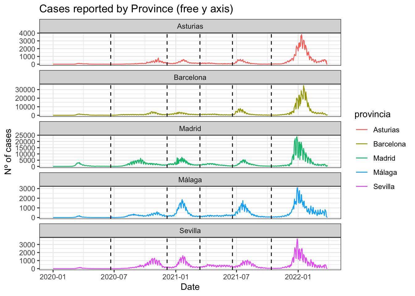
The incidence of Covid-19 in Madrid and Barcelona are much larger than in the rest of the provinces, mainly due to the number of inhabitants. The next figure show the same information than the previous one but freeing the y-axis scale.

This approach will be followed in further plots.

covid_data %>% 
      ggplot(aes(x = fecha, y = num_casos)) +
      geom_line(aes(color = provincia)) +
      geom_vline(xintercept = as.Date("2020-06-21", format = "%Y-%m-%d"), linetype="dashed") +
      geom_vline(xintercept = as.Date("2020-12-06", format = "%Y-%m-%d"), linetype="dashed") +
      geom_vline(xintercept = as.Date("2021-03-14", format = "%Y-%m-%d"), linetype="dashed") +
      geom_vline(xintercept = as.Date("2021-06-19", format = "%Y-%m-%d"), linetype="dashed") +
      geom_vline(xintercept = as.Date("2021-10-13", format = "%Y-%m-%d"), linetype="dashed") +
      facet_wrap(~provincia, scales = "free_y", ncol=1) +
      theme(legend.position = "top") +
      labs(title="Cases reported by Province (free y axis)",
           x ="Date", y = "Nº of cases") +
      theme_bw()

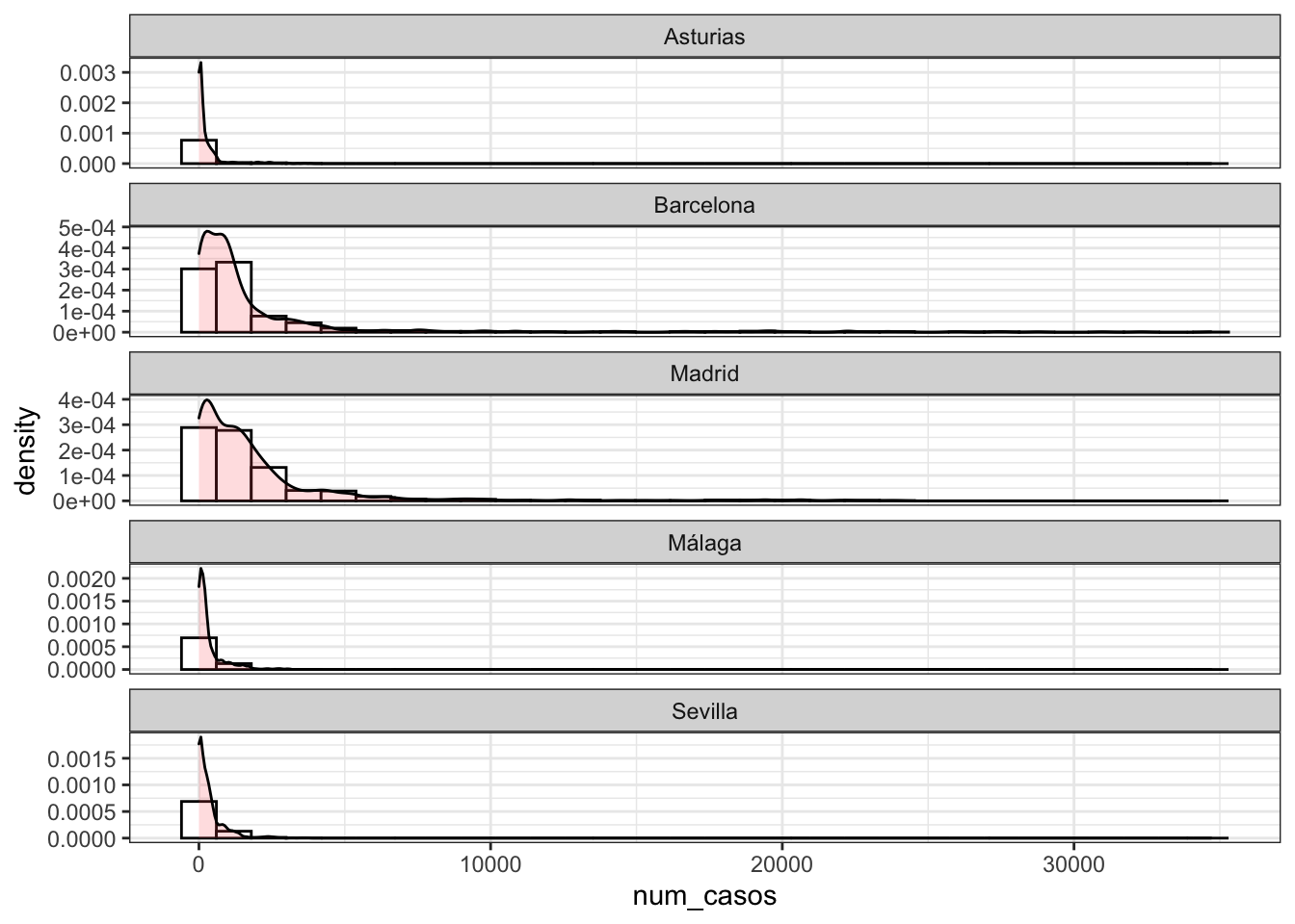
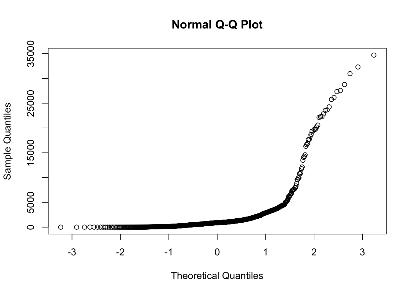
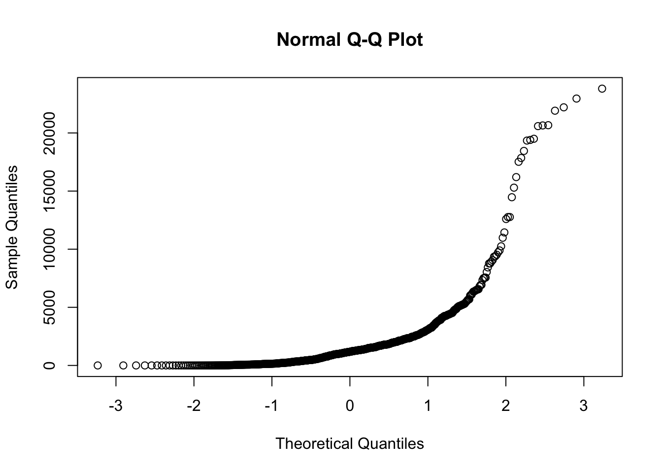
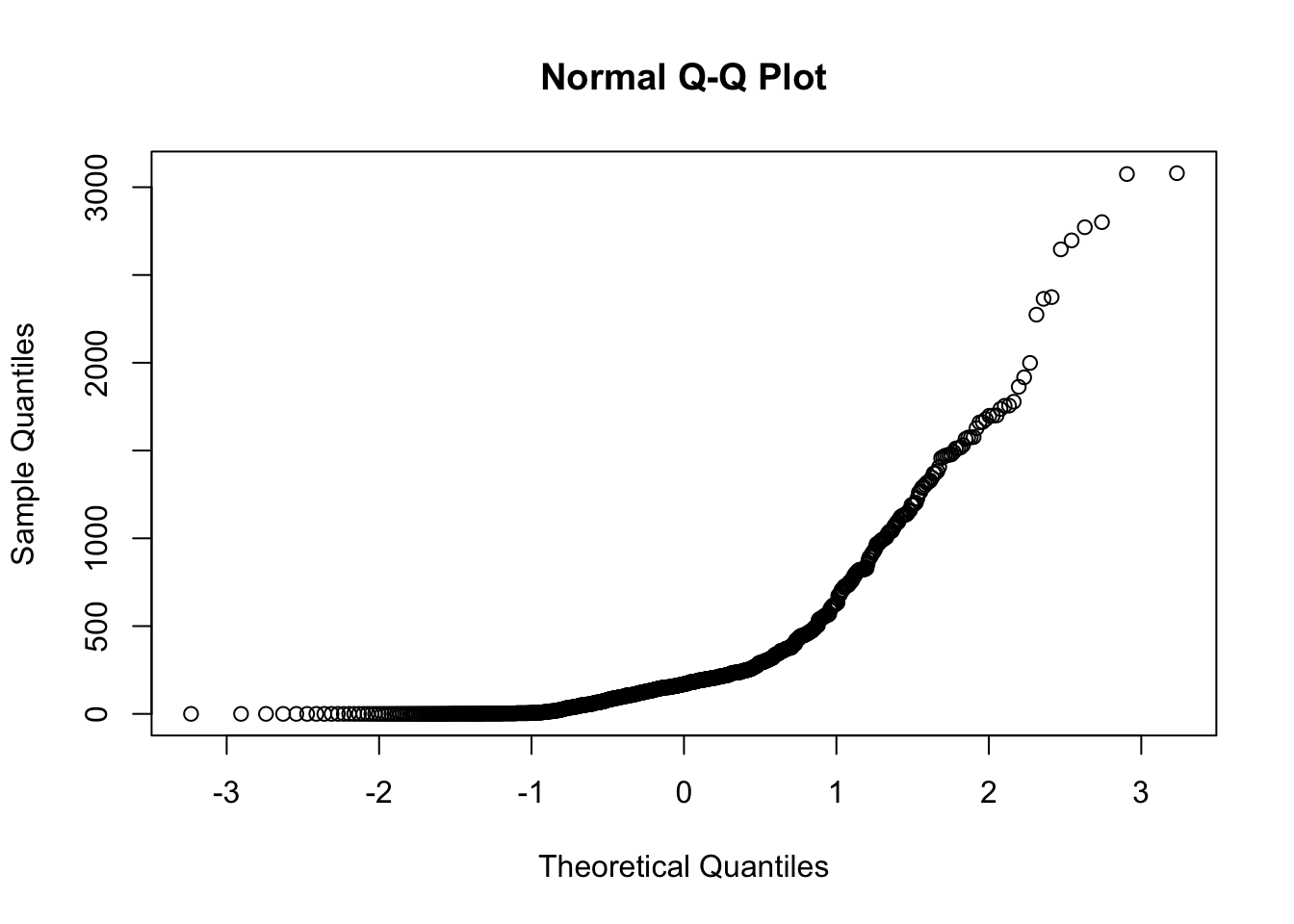
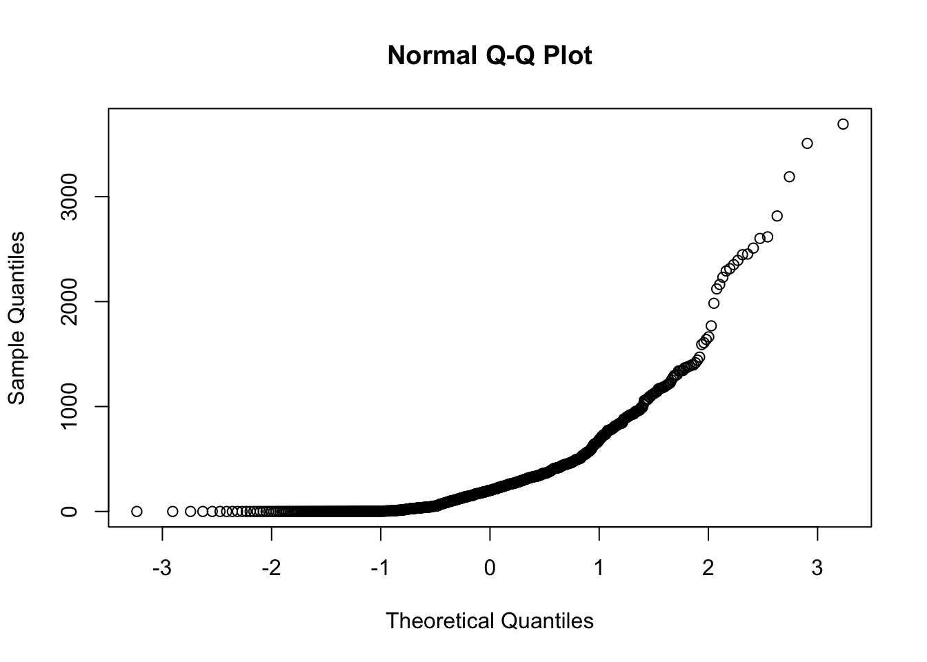
Normality study

# Histogram with density plot
covid_data %>% 
      ggplot(aes(x=num_casos)) + 
      geom_histogram(aes(y=..density..), colour="black", fill="white")+
      geom_density(alpha=.2, fill="#FF6666") +
      facet_wrap(~provincia, scales = "free_y", ncol=1) +
      theme_bw()

covid_data %>% 
      filter(provincia == "Asturias") %>% 
      pull(num_casos) %>% 
      qqnorm()

covid_data %>% 
      filter(provincia == "Barcelona") %>% 
      pull(num_casos) %>% 
      qqnorm()

covid_data %>% 
      filter(provincia == "Madrid") %>% 
      pull(num_casos) %>% 
      qqnorm()

covid_data %>% 
      filter(provincia == "Málaga") %>% 
      pull(num_casos) %>% 
      qqnorm()

covid_data %>% 
      filter(provincia == "Sevilla") %>% 
      pull(num_casos) %>% 
      qqnorm()

Number of PCR positives:

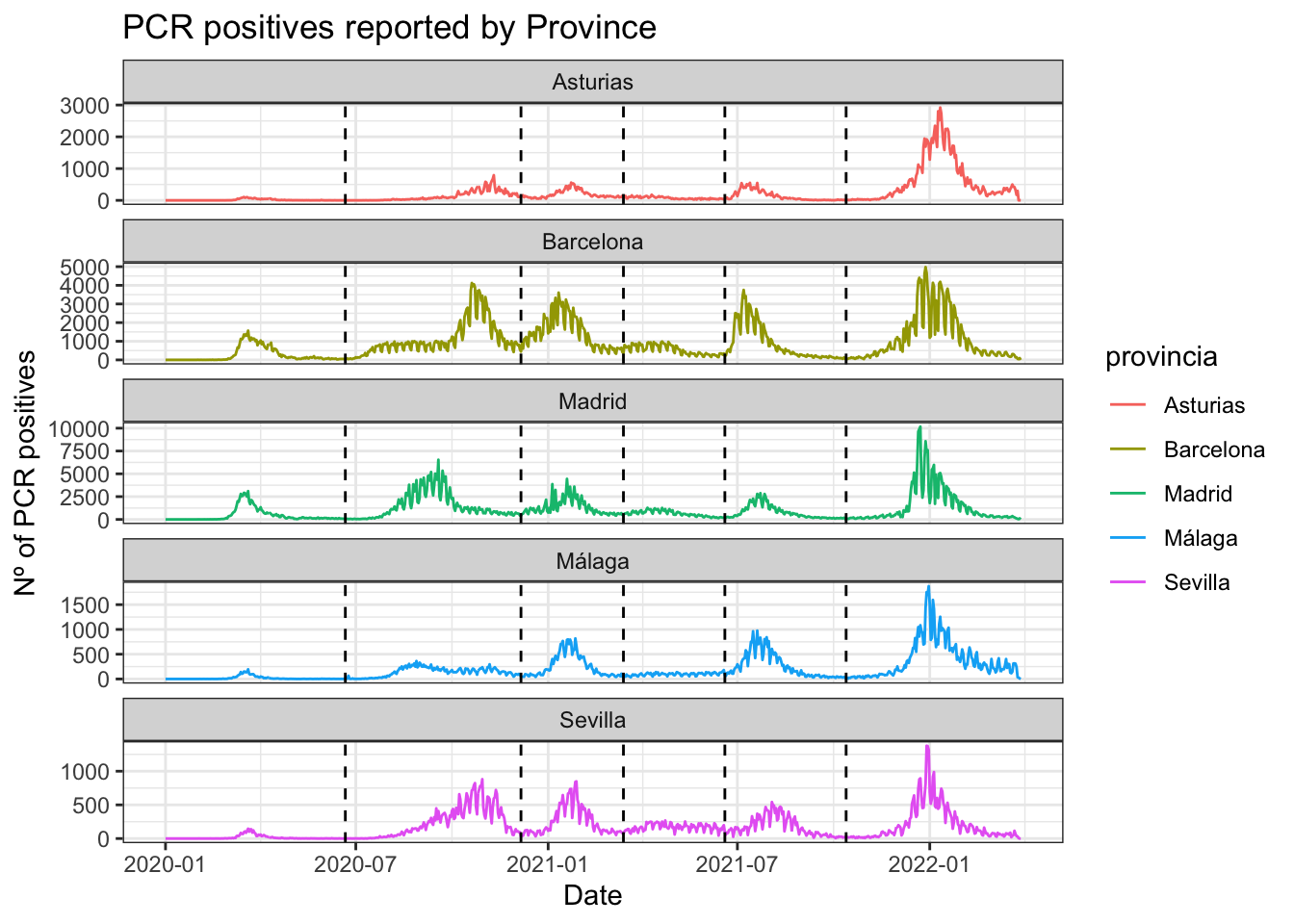
covid_data %>% 
      ggplot(aes(x = fecha)) +
      geom_line(aes(y = num_casos_prueba_pcr, color = provincia)) +
      geom_vline(xintercept = as.Date("2020-06-21", format = "%Y-%m-%d"), linetype="dashed") +
      geom_vline(xintercept = as.Date("2020-12-06", format = "%Y-%m-%d"), linetype="dashed") +
      geom_vline(xintercept = as.Date("2021-03-14", format = "%Y-%m-%d"), linetype="dashed") +
      geom_vline(xintercept = as.Date("2021-06-19", format = "%Y-%m-%d"), linetype="dashed") +
      geom_vline(xintercept = as.Date("2021-10-13", format = "%Y-%m-%d"), linetype="dashed") +
      facet_wrap(~provincia, scales = "free_y", ncol=1) +
      theme(legend.position = "top") +
      labs(title="PCR positives reported by Province",
           x ="Date", y = "Nº of PCR positives") +
      theme_bw()

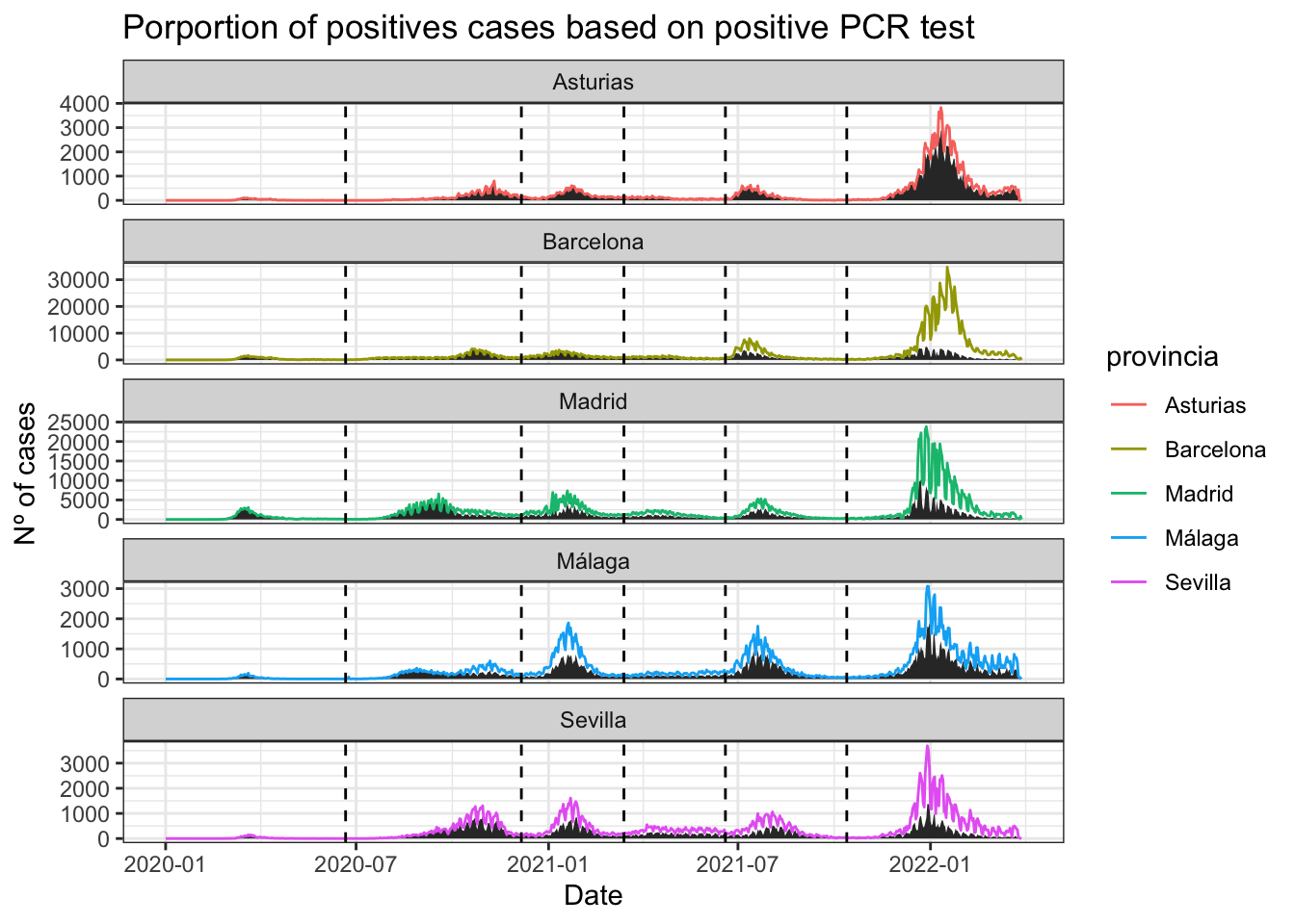
Number of covid cases accounted by positive PCR tests:

covid_data %>% 
      ggplot(aes(x = fecha)) +
      geom_area(aes(y = num_casos_prueba_pcr)) +
      geom_line(aes(y = num_casos, color = provincia)) +
      geom_vline(xintercept = as.Date("2020-06-21", format = "%Y-%m-%d"), linetype="dashed") +
      geom_vline(xintercept = as.Date("2020-12-06", format = "%Y-%m-%d"), linetype="dashed") +
      geom_vline(xintercept = as.Date("2021-03-14", format = "%Y-%m-%d"), linetype="dashed") +
      geom_vline(xintercept = as.Date("2021-06-19", format = "%Y-%m-%d"), linetype="dashed") +
      geom_vline(xintercept = as.Date("2021-10-13", format = "%Y-%m-%d"), linetype="dashed") +
      facet_wrap(~provincia, scales = "free_y", ncol=1) +
      theme(legend.position = "top") +
      labs(title="Porportion of positives cases based on positive PCR test",
           x ="Date", y = "Nº of cases") +
      theme_bw()

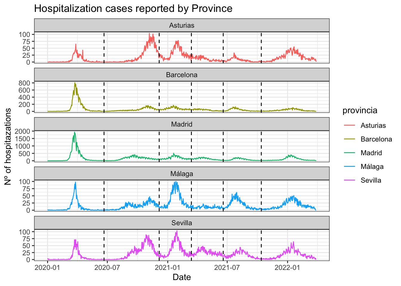
Number of hospitalizations:

covid_data %>% 
      ggplot() +
      geom_line(aes(x = fecha, y = num_hosp, color = provincia)) +
      geom_vline(xintercept = as.Date("2020-06-21", format = "%Y-%m-%d"), linetype="dashed") +
      geom_vline(xintercept = as.Date("2020-12-06", format = "%Y-%m-%d"), linetype="dashed") +
      geom_vline(xintercept = as.Date("2021-03-14", format = "%Y-%m-%d"), linetype="dashed") +
      geom_vline(xintercept = as.Date("2021-06-19", format = "%Y-%m-%d"), linetype="dashed") +
      geom_vline(xintercept = as.Date("2021-10-13", format = "%Y-%m-%d"), linetype="dashed") +
      facet_wrap(~provincia, scales = "free_y", ncol=1) +
      theme(legend.position = "top") +
      labs(title="Hospitalization cases reported by Province",
           x ="Date", y = "Nº of hospitazations") +
      theme_bw()

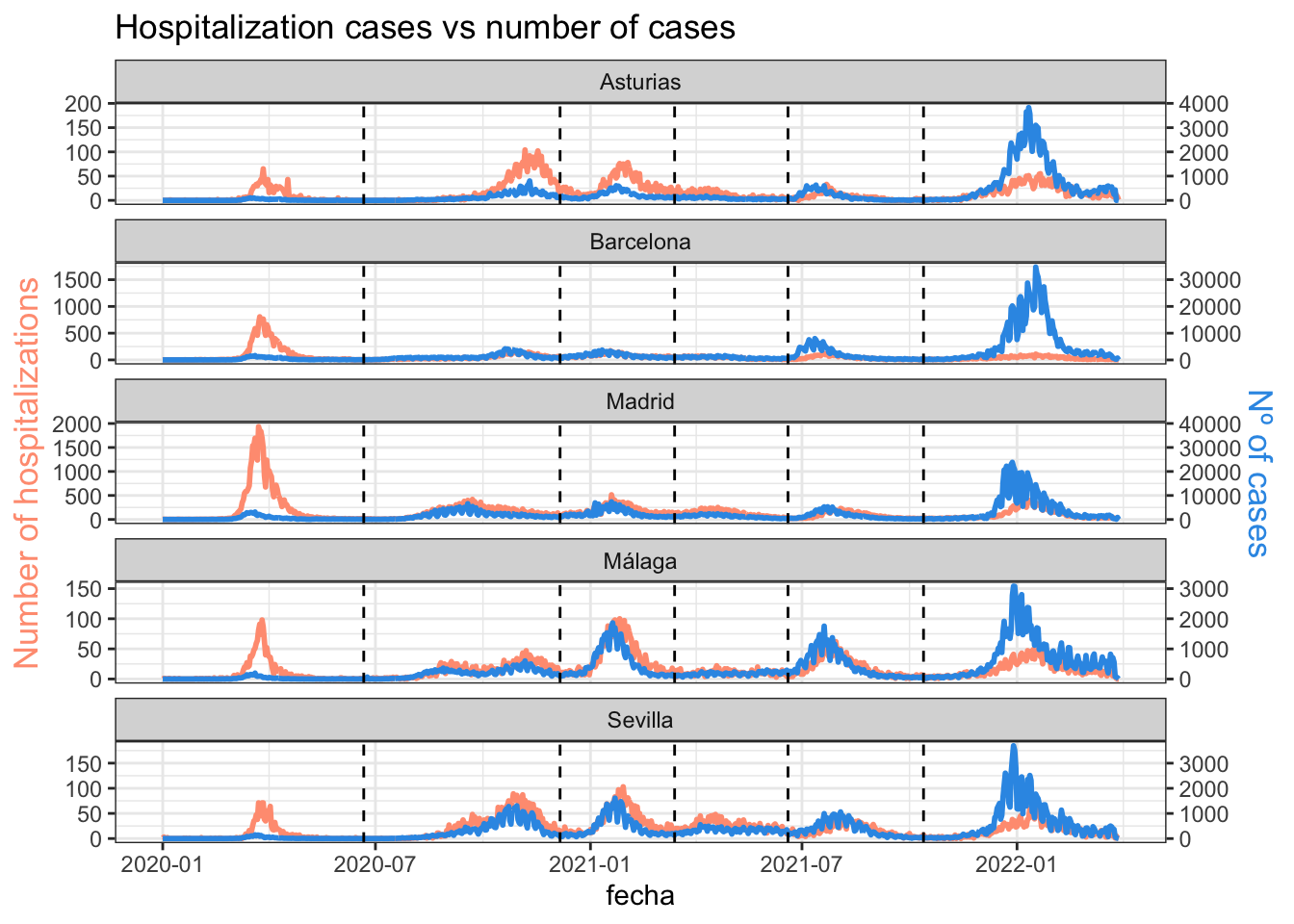
Number of hospitalizations vs number of cases:

# Value used to transform the data
coeff <- 20

# A few constants for colors
temperatureColor <- "#ff9e81"
priceColor <- rgb(0.2, 0.6, 0.9, 1)

covid_data %>% 
      ggplot(aes(x = fecha)) +
      geom_line( aes(y = num_hosp), size=1, color=temperatureColor) + 
      geom_line( aes(y = num_casos / coeff), size=1, color=priceColor) +
      geom_vline(xintercept = as.Date("2020-06-21", format = "%Y-%m-%d"), linetype="dashed") +
      geom_vline(xintercept = as.Date("2020-12-06", format = "%Y-%m-%d"), linetype="dashed") +
      geom_vline(xintercept = as.Date("2021-03-14", format = "%Y-%m-%d"), linetype="dashed") +
      geom_vline(xintercept = as.Date("2021-06-19", format = "%Y-%m-%d"), linetype="dashed") +
      geom_vline(xintercept = as.Date("2021-10-13", format = "%Y-%m-%d"), linetype="dashed") +
      scale_y_continuous(
            # Features of the first axis
            name = "Number of hospitalizations",
            # Add a second axis and specify its features
            sec.axis = sec_axis(~.*coeff, name="Nº of cases")
      ) +
      facet_wrap(~provincia, scales = "free_y", ncol=1) +
      theme_bw() +
      theme(
            axis.title.y = element_text(color = temperatureColor, size=13),
            axis.title.y.right = element_text(color = priceColor, size=13)
      ) +
      ggtitle("Hospitalization cases vs number of cases")

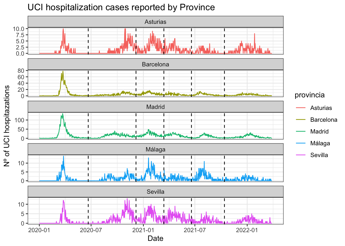
Number of UCI hospitalizations:

covid_data %>% 
      ggplot() +
      geom_line(aes(x = fecha, y = num_uci, color = provincia)) +
      geom_vline(xintercept = as.Date("2020-06-21", format = "%Y-%m-%d"), linetype="dashed") +
      geom_vline(xintercept = as.Date("2020-12-06", format = "%Y-%m-%d"), linetype="dashed") +
      geom_vline(xintercept = as.Date("2021-03-14", format = "%Y-%m-%d"), linetype="dashed") +
      geom_vline(xintercept = as.Date("2021-06-19", format = "%Y-%m-%d"), linetype="dashed") +
      geom_vline(xintercept = as.Date("2021-10-13", format = "%Y-%m-%d"), linetype="dashed") +
      facet_wrap(~provincia, scales = "free_y", ncol=1) +
      theme(legend.position = "top") +
      labs(title="UCI hospitalization cases reported by Province",
           x ="Date", y = "Nº of UCI hospitazations") +
      theme_bw()

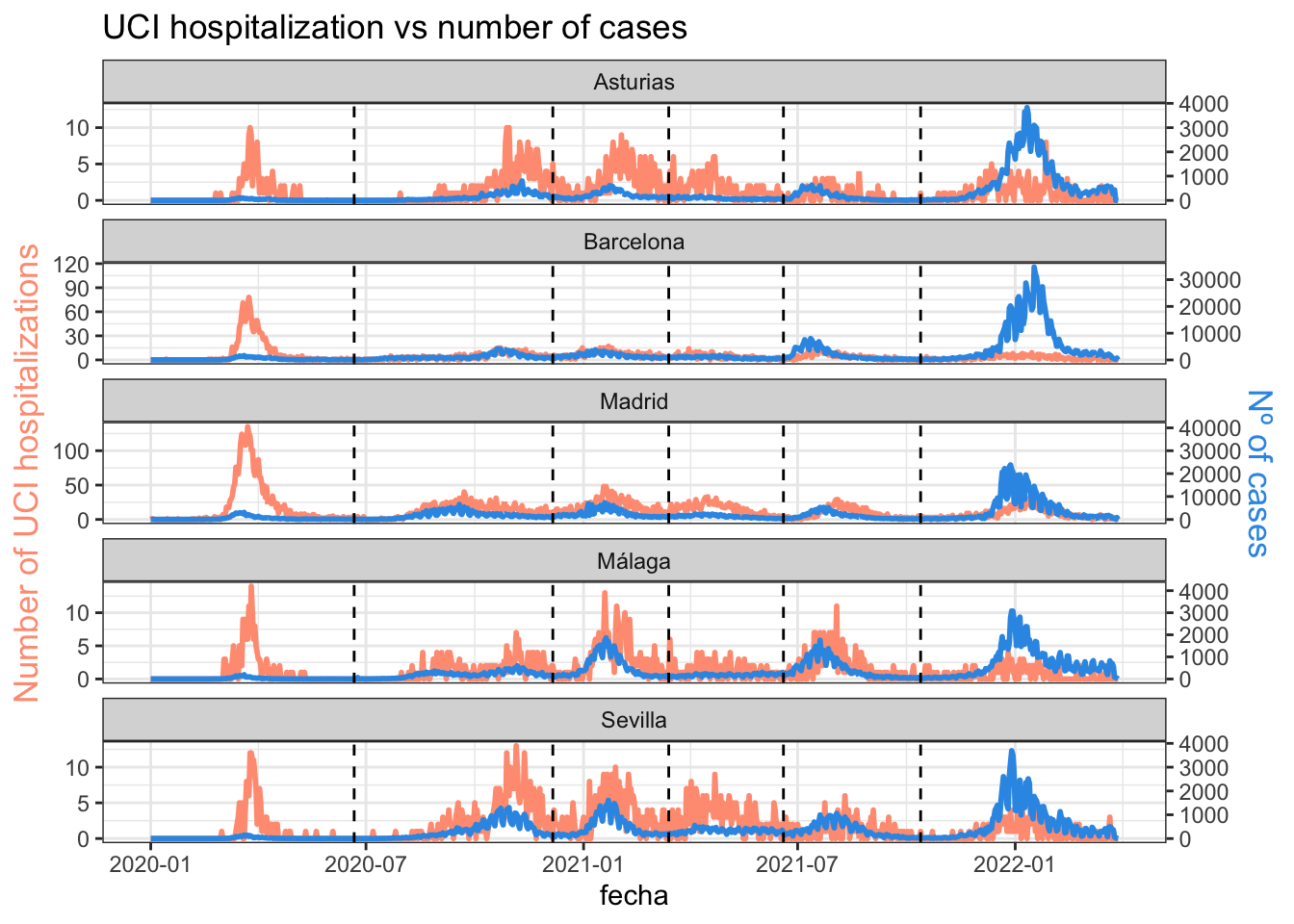
Number of UCI hospitalizations vs number of cases:

# Value used to transform the data
coeff <- 300

# A few constants for colors
temperatureColor <- "#ff9e81"
priceColor <- rgb(0.2, 0.6, 0.9, 1)

covid_data %>% 
      ggplot(aes(x = fecha)) +
      geom_line( aes(y = num_uci), size=1, color=temperatureColor) + 
      geom_line( aes(y = num_casos / coeff), size=1, color=priceColor) +
      geom_vline(xintercept = as.Date("2020-06-21", format = "%Y-%m-%d"), linetype="dashed") +
      geom_vline(xintercept = as.Date("2020-12-06", format = "%Y-%m-%d"), linetype="dashed") +
      geom_vline(xintercept = as.Date("2021-03-14", format = "%Y-%m-%d"), linetype="dashed") +
      geom_vline(xintercept = as.Date("2021-06-19", format = "%Y-%m-%d"), linetype="dashed") +
      geom_vline(xintercept = as.Date("2021-10-13", format = "%Y-%m-%d"), linetype="dashed") +
      scale_y_continuous(
            # Features of the first axis
            name = "Number of UCI hospitalizations",
            # Add a second axis and specify its features
            sec.axis = sec_axis(~.*coeff, name="Nº of cases")
      ) +
      facet_wrap(~provincia, scales = "free_y", ncol=1) +
      theme_bw() +
      theme(
            axis.title.y = element_text(color = temperatureColor, size=13),
            axis.title.y.right = element_text(color = priceColor, size=13)
      ) +
      ggtitle("UCI hospitalization vs number of cases")

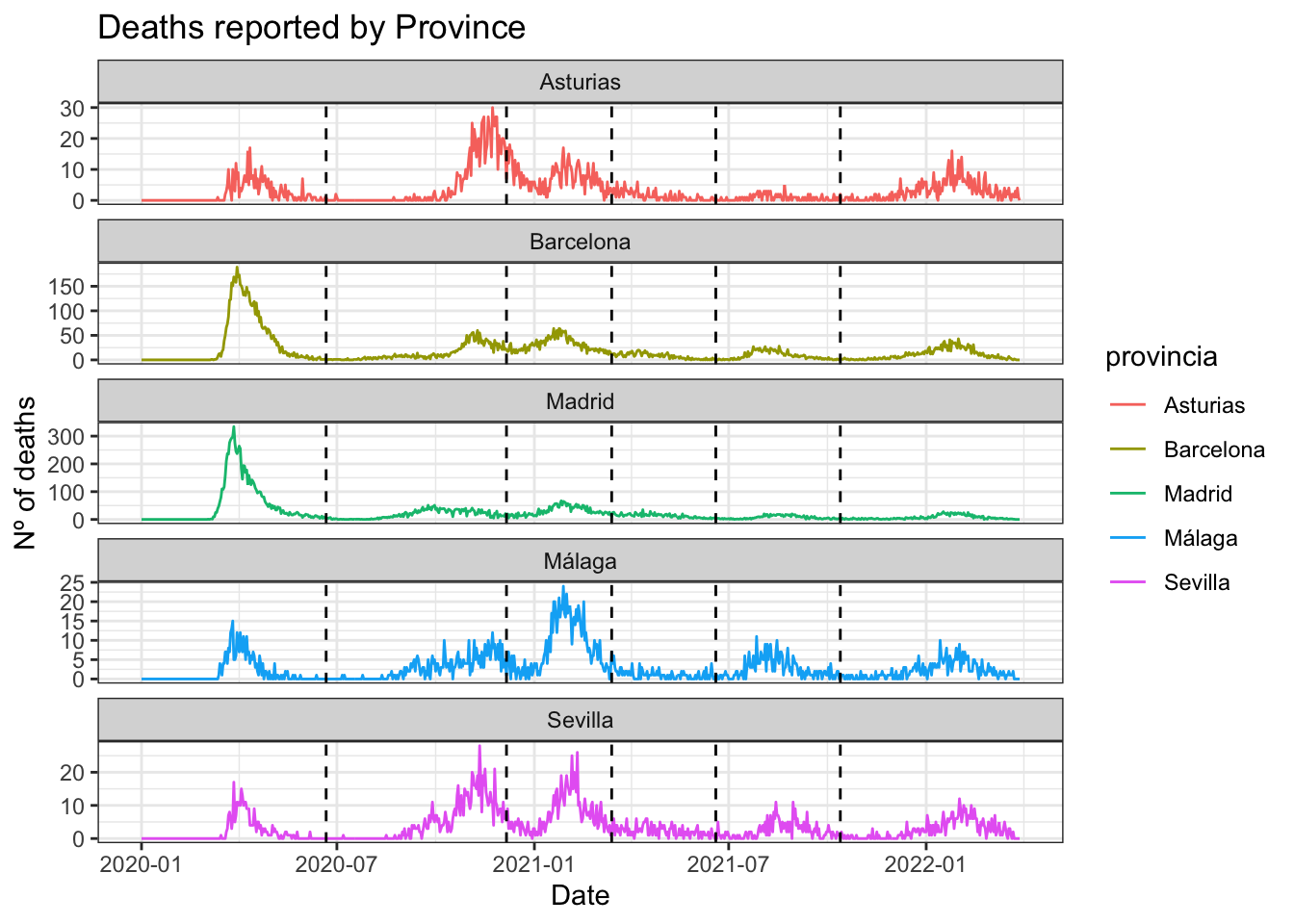
Number of deaths

covid_data %>% 
      ggplot() +
      geom_line(aes(x = fecha, y = num_def, color = provincia)) +
      geom_vline(xintercept = as.Date("2020-06-21", format = "%Y-%m-%d"), linetype="dashed") +
      geom_vline(xintercept = as.Date("2020-12-06", format = "%Y-%m-%d"), linetype="dashed") +
      geom_vline(xintercept = as.Date("2021-03-14", format = "%Y-%m-%d"), linetype="dashed") +
      geom_vline(xintercept = as.Date("2021-06-19", format = "%Y-%m-%d"), linetype="dashed") +
      geom_vline(xintercept = as.Date("2021-10-13", format = "%Y-%m-%d"), linetype="dashed") +
      facet_wrap(~provincia, scales = "free_y", ncol=1) +
      theme(legend.position = "top") +
      labs(title="Deaths reported by Province",
           x ="Date", y = "Nº of deaths") +
      theme_bw()

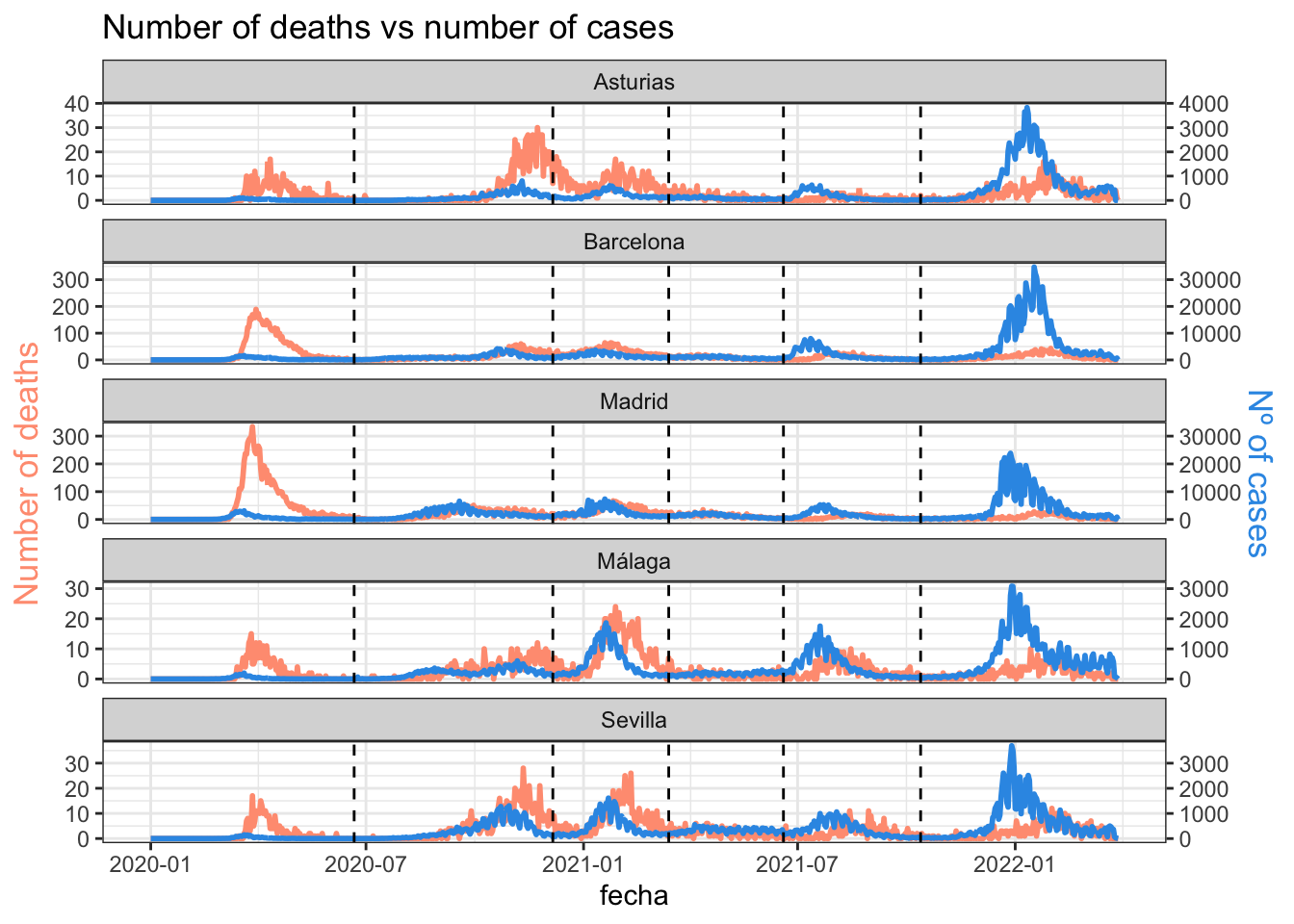
# Value used to transform the data
coeff <- 100

# A few constants for colors
temperatureColor <- "#ff9e81"
priceColor <- rgb(0.2, 0.6, 0.9, 1)

covid_data %>% 
      ggplot(aes(x = fecha)) +
      geom_line( aes(y = num_def), size=1, color=temperatureColor) + 
      geom_line( aes(y = num_casos / coeff), size=1, color=priceColor) +
      geom_vline(xintercept = as.Date("2020-06-21", format = "%Y-%m-%d"), linetype="dashed") +
      geom_vline(xintercept = as.Date("2020-12-06", format = "%Y-%m-%d"), linetype="dashed") +
      geom_vline(xintercept = as.Date("2021-03-14", format = "%Y-%m-%d"), linetype="dashed") +
      geom_vline(xintercept = as.Date("2021-06-19", format = "%Y-%m-%d"), linetype="dashed") +
      geom_vline(xintercept = as.Date("2021-10-13", format = "%Y-%m-%d"), linetype="dashed") +
      scale_y_continuous(
            # Features of the first axis
            name = "Number of deaths",
            # Add a second axis and specify its features
            sec.axis = sec_axis(~.*coeff, name="Nº of cases")
      ) +
      facet_wrap(~provincia, scales = "free_y", ncol=1) +
      theme_bw() +
      theme(
            axis.title.y = element_text(color = temperatureColor, size=13),
            axis.title.y.right = element_text(color = priceColor, size=13)
      ) +
      ggtitle("Number of deaths vs number of cases")

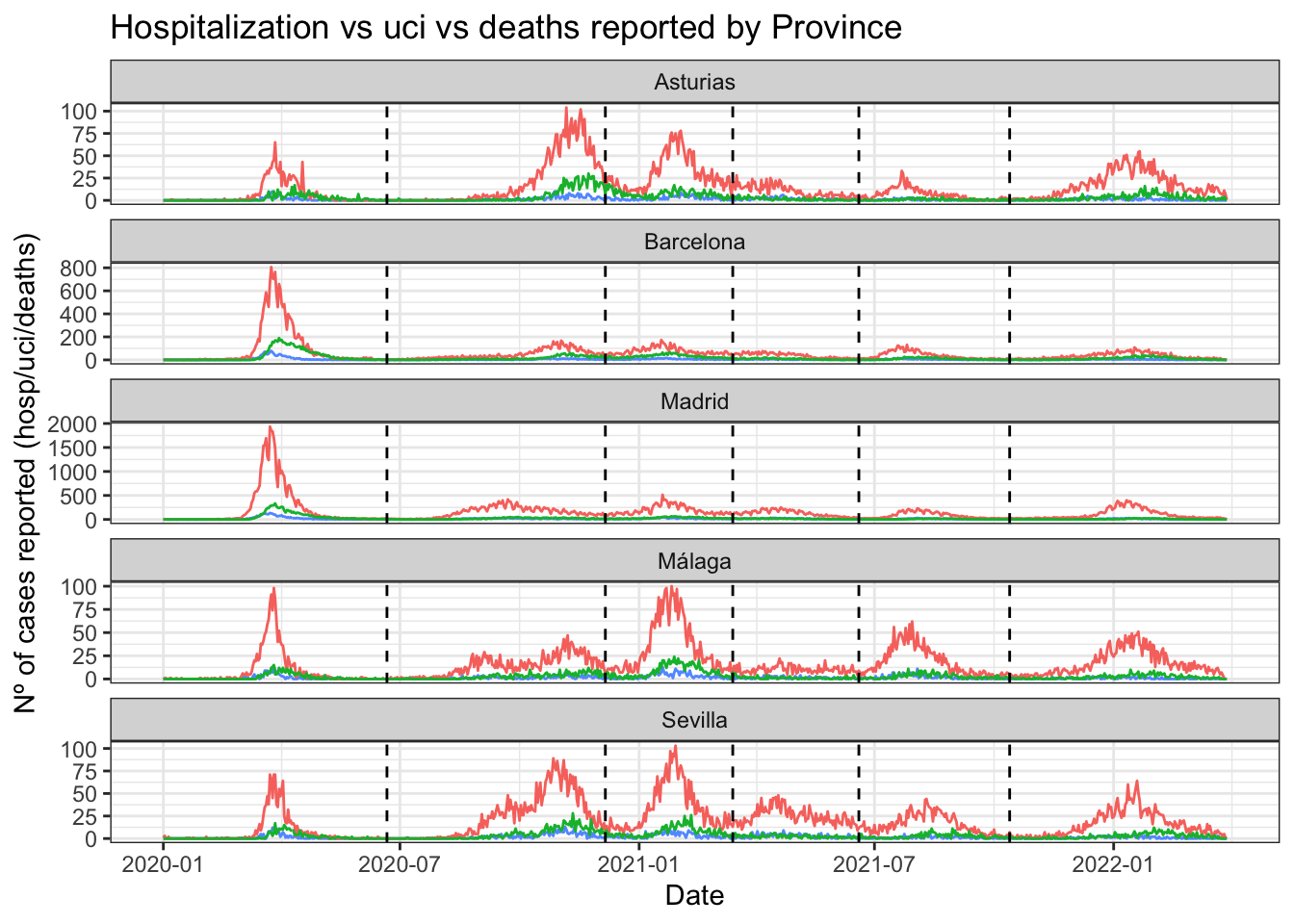
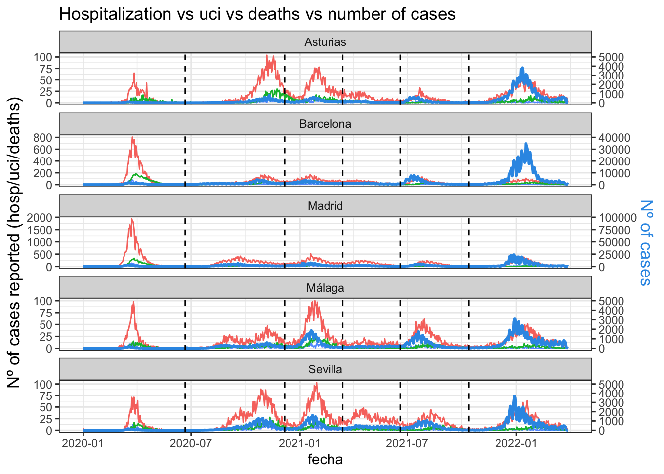
hospitalizations vs uci vs deaths

covid_data %>% 
      ggplot() +
      # geom_line(aes(x = fecha, y = num_uci, color = provincia)) +
      # geom_line(aes(x = fecha, y = num_hosp, color = provincia)) +
      # geom_line(aes(x = fecha, y = num_def, color = provincia)) +
      geom_line(aes(x = fecha, y = num_uci, color = "red")) +
      geom_line(aes(x = fecha, y = num_hosp, color = "black")) +
      geom_line(aes(x = fecha, y = num_def, color = "blue")) +
      geom_vline(xintercept = as.Date("2020-06-21", format = "%Y-%m-%d"), linetype="dashed") +
      geom_vline(xintercept = as.Date("2020-12-06", format = "%Y-%m-%d"), linetype="dashed") +
      geom_vline(xintercept = as.Date("2021-03-14", format = "%Y-%m-%d"), linetype="dashed") +
      geom_vline(xintercept = as.Date("2021-06-19", format = "%Y-%m-%d"), linetype="dashed") +
      geom_vline(xintercept = as.Date("2021-10-13", format = "%Y-%m-%d"), linetype="dashed") +
      facet_wrap(~provincia, scales = "free_y", ncol=1) +
      theme(legend.position = "top") +
      labs(title="Hospitalization vs uci vs deaths reported by Province",
           x ="Date", y = "Nº of cases reported (hosp/uci/deaths)") +
      theme_bw() +
      theme(legend.position = "none") 

# Value used to transform the data
coeff <- 50

# A few constants for colors
priceColor <- rgb(0.2, 0.6, 0.9, 1)

covid_data %>% 
      ggplot(aes(x = fecha)) +
      geom_line(aes(x = fecha, y = num_uci, color = "red")) +
      geom_line(aes(x = fecha, y = num_hosp, color = "black")) +
      geom_line(aes(x = fecha, y = num_def, color = "blue")) +
      geom_line( aes(y = num_casos / coeff), size=1, color=priceColor) +
      geom_vline(xintercept = as.Date("2020-06-21", format = "%Y-%m-%d"), linetype="dashed") +
      geom_vline(xintercept = as.Date("2020-12-06", format = "%Y-%m-%d"), linetype="dashed") +
      geom_vline(xintercept = as.Date("2021-03-14", format = "%Y-%m-%d"), linetype="dashed") +
      geom_vline(xintercept = as.Date("2021-06-19", format = "%Y-%m-%d"), linetype="dashed") +
      geom_vline(xintercept = as.Date("2021-10-13", format = "%Y-%m-%d"), linetype="dashed") +
      scale_y_continuous(
            # Features of the first axis
            name = "Nº of cases reported (hosp/uci/deaths)",
            # Add a second axis and specify its features
            sec.axis = sec_axis(~.*coeff, name="Nº of cases")
      ) +
      facet_wrap(~provincia, scales = "free_y", ncol=1) +
      theme_bw() +
      theme(
            axis.title.y = element_text(size=13),
            axis.title.y.right = element_text(color = priceColor, size=13),
            legend.position = "none") +
      ggtitle("Hospitalization vs uci vs deaths vs number of cases")

Meteorology

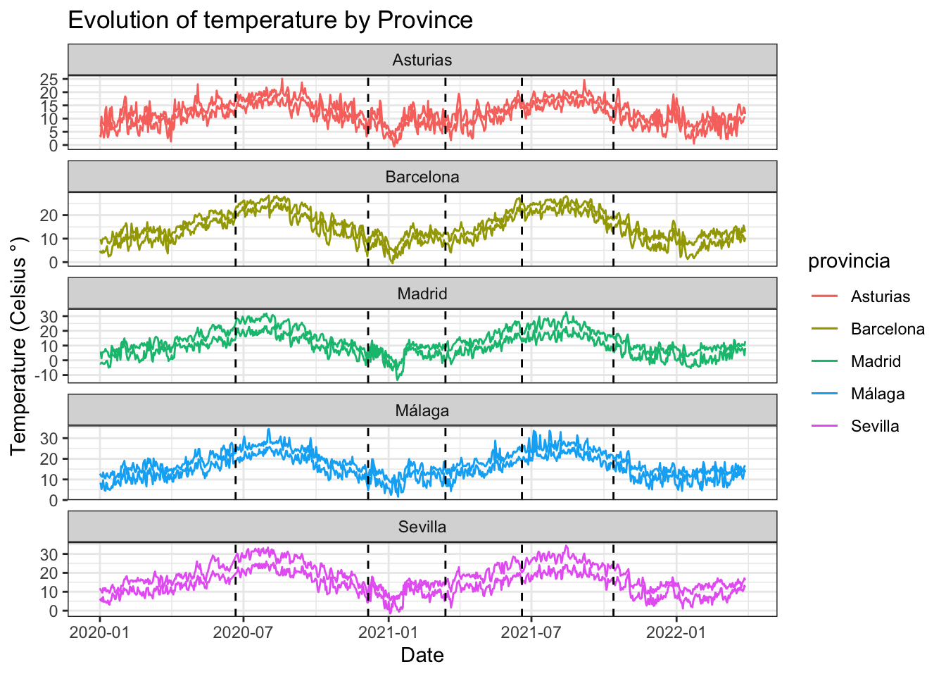
tmed vs tmin

covid_data %>% 
      ggplot(aes(x = fecha)) +
      geom_line(aes(y = tmed, color = provincia)) +
      geom_line(aes(y = tmin, color = provincia)) +
      geom_vline(xintercept = as.Date("2020-06-21", format = "%Y-%m-%d"), linetype="dashed") +
      geom_vline(xintercept = as.Date("2020-12-06", format = "%Y-%m-%d"), linetype="dashed") +
      geom_vline(xintercept = as.Date("2021-03-14", format = "%Y-%m-%d"), linetype="dashed") +
      geom_vline(xintercept = as.Date("2021-06-19", format = "%Y-%m-%d"), linetype="dashed") +
      geom_vline(xintercept = as.Date("2021-10-13", format = "%Y-%m-%d"), linetype="dashed") +
      facet_wrap(~provincia, scales = "free_y", ncol=1) +
      theme(legend.position = "top") +
      labs(title="Evolution of temperature by Province",
           x ="Date", y = "Temperature (Celsius °)") +
      theme_bw()

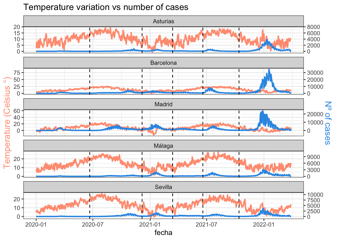
Evolution of temperature vs number cases:

# Value used to transform the data
coeff <- 400

# A few constants for colors
temperatureColor <- "#ff9e81"
priceColor <- rgb(0.2, 0.6, 0.9, 1)

covid_data %>% 
      ggplot(aes(x = fecha)) +
      geom_line( aes(y = tmin), size=1, color=temperatureColor) + 
      geom_line( aes(y = num_casos / coeff), size=1, color=priceColor) +
      geom_vline(xintercept = as.Date("2020-06-21", format = "%Y-%m-%d"), linetype="dashed") +
      geom_vline(xintercept = as.Date("2020-12-06", format = "%Y-%m-%d"), linetype="dashed") +
      geom_vline(xintercept = as.Date("2021-03-14", format = "%Y-%m-%d"), linetype="dashed") +
      geom_vline(xintercept = as.Date("2021-06-19", format = "%Y-%m-%d"), linetype="dashed") +
      geom_vline(xintercept = as.Date("2021-10-13", format = "%Y-%m-%d"), linetype="dashed") +
      scale_y_continuous(
            # Features of the first axis
            name = "Temperature (Celsius °)",
            # Add a second axis and specify its features
            sec.axis = sec_axis(~.*coeff, name="Nº of cases")
      ) +
      facet_wrap(~provincia, scales = "free_y", ncol=1) +
      theme_bw() +
      theme(
            axis.title.y = element_text(color = temperatureColor, size=13),
            axis.title.y.right = element_text(color = priceColor, size=13)
      ) +
      ggtitle("Temperature variation vs number of cases")

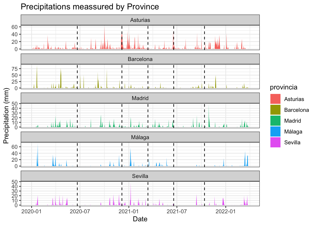
Precipitations

covid_data %>% 
      ggplot(aes(x = fecha)) +
      geom_area(aes(y = prec, fill = provincia)) +
      geom_vline(xintercept = as.Date("2020-06-21", format = "%Y-%m-%d"), linetype="dashed") +
      geom_vline(xintercept = as.Date("2020-12-06", format = "%Y-%m-%d"), linetype="dashed") +
      geom_vline(xintercept = as.Date("2021-03-14", format = "%Y-%m-%d"), linetype="dashed") +
      geom_vline(xintercept = as.Date("2021-06-19", format = "%Y-%m-%d"), linetype="dashed") +
      geom_vline(xintercept = as.Date("2021-10-13", format = "%Y-%m-%d"), linetype="dashed") +
      facet_wrap(~provincia, scales = "free_y", ncol=1) +
      theme(legend.position = "top") +
      labs(title="Precipitations meassured by Province",
           x ="Date", y = "Precipitation (mm)") +
      theme_bw()

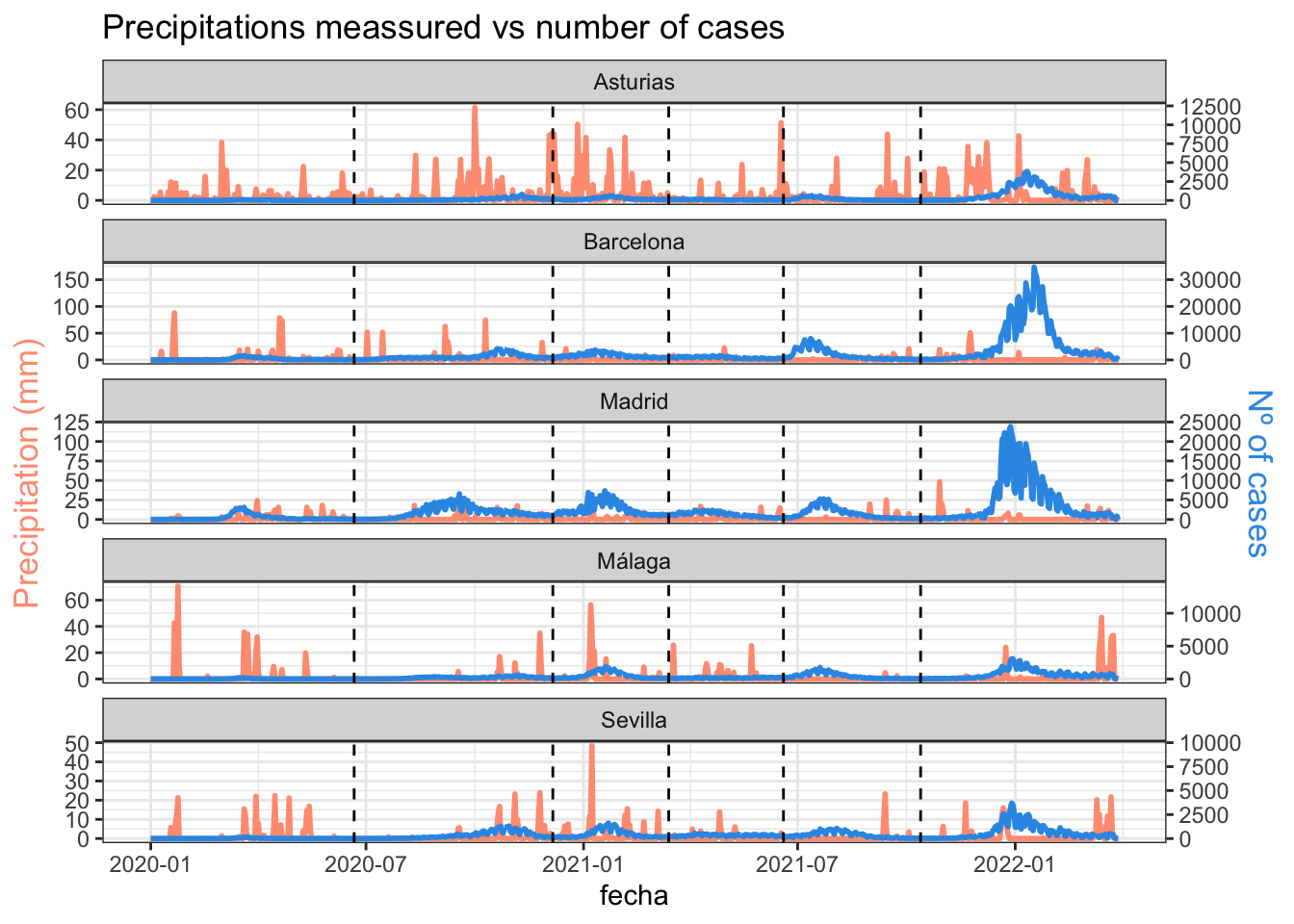
Precipitations vs number cases:

# Value used to transform the data
coeff <- 200

# A few constants for colors
temperatureColor <- "#ff9e81"
priceColor <- rgb(0.2, 0.6, 0.9, 1)

covid_data %>% 
      ggplot(aes(x = fecha)) +
      geom_line( aes(y = prec), size=1, color=temperatureColor) + 
      geom_line( aes(y = num_casos / coeff), size=1, color=priceColor) +
      geom_vline(xintercept = as.Date("2020-06-21", format = "%Y-%m-%d"), linetype="dashed") +
      geom_vline(xintercept = as.Date("2020-12-06", format = "%Y-%m-%d"), linetype="dashed") +
      geom_vline(xintercept = as.Date("2021-03-14", format = "%Y-%m-%d"), linetype="dashed") +
      geom_vline(xintercept = as.Date("2021-06-19", format = "%Y-%m-%d"), linetype="dashed") +
      geom_vline(xintercept = as.Date("2021-10-13", format = "%Y-%m-%d"), linetype="dashed") +
      scale_y_continuous(
            # Features of the first axis
            name = "Precipitation (mm)",
            # Add a second axis and specify its features
            sec.axis = sec_axis(~.*coeff, name="Nº of cases")
      ) +
      facet_wrap(~provincia, scales = "free_y", ncol=1) +
      theme_bw() +
      theme(
            axis.title.y = element_text(color = temperatureColor, size=13),
            axis.title.y.right = element_text(color = priceColor, size=13)
      ) +
      ggtitle("Precipitations meassured vs number of cases")

Mobility

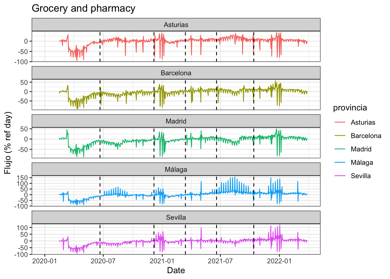
grocery and pharmacy

covid_data %>% 
      ggplot(aes(x = fecha)) +
      geom_line(aes(y = mob_grocery_pharmacy, color = provincia)) +
      geom_vline(xintercept = as.Date("2020-06-21", format = "%Y-%m-%d"), linetype="dashed") +
      geom_vline(xintercept = as.Date("2020-12-06", format = "%Y-%m-%d"), linetype="dashed") +
      geom_vline(xintercept = as.Date("2021-03-14", format = "%Y-%m-%d"), linetype="dashed") +
      geom_vline(xintercept = as.Date("2021-06-19", format = "%Y-%m-%d"), linetype="dashed") +
      geom_vline(xintercept = as.Date("2021-10-13", format = "%Y-%m-%d"), linetype="dashed") +
      facet_wrap(~provincia, scales = "free_y", ncol=1) +
      theme(legend.position = "top") +
      labs(title="Grocery and pharmacy",
           x ="Date", y = "Flujo (% ref day)") +
      theme_bw()

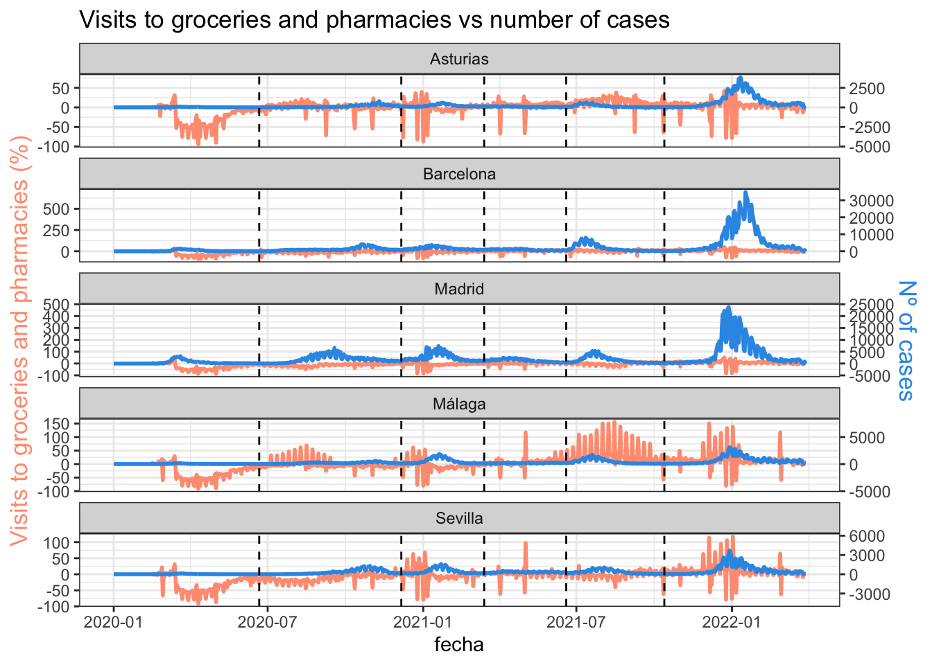
# Value used to transform the data
coeff <- 50

# A few constants for colors
temperatureColor <- "#ff9e81"
priceColor <- rgb(0.2, 0.6, 0.9, 1)

covid_data %>% 
      ggplot(aes(x = fecha)) +
      geom_line( aes(y = mob_grocery_pharmacy), size=1, color=temperatureColor) + 
      geom_line( aes(y = num_casos / coeff), size=1, color=priceColor) +
      geom_vline(xintercept = as.Date("2020-06-21", format = "%Y-%m-%d"), linetype="dashed") +
      geom_vline(xintercept = as.Date("2020-12-06", format = "%Y-%m-%d"), linetype="dashed") +
      geom_vline(xintercept = as.Date("2021-03-14", format = "%Y-%m-%d"), linetype="dashed") +
      geom_vline(xintercept = as.Date("2021-06-19", format = "%Y-%m-%d"), linetype="dashed") +
      geom_vline(xintercept = as.Date("2021-10-13", format = "%Y-%m-%d"), linetype="dashed") +
      scale_y_continuous(
            # Features of the first axis
            name = "Visits to groceries and pharmacies (%)",
            # Add a second axis and specify its features
            sec.axis = sec_axis(~.*coeff, name="Nº of cases")
      ) +
      facet_wrap(~provincia, scales = "free_y", ncol=1) +
      theme_bw() +
      theme(
            axis.title.y = element_text(color = temperatureColor, size=13),
            axis.title.y.right = element_text(color = priceColor, size=13)
      ) +
      ggtitle("Visits to groceries and pharmacies vs number of cases")

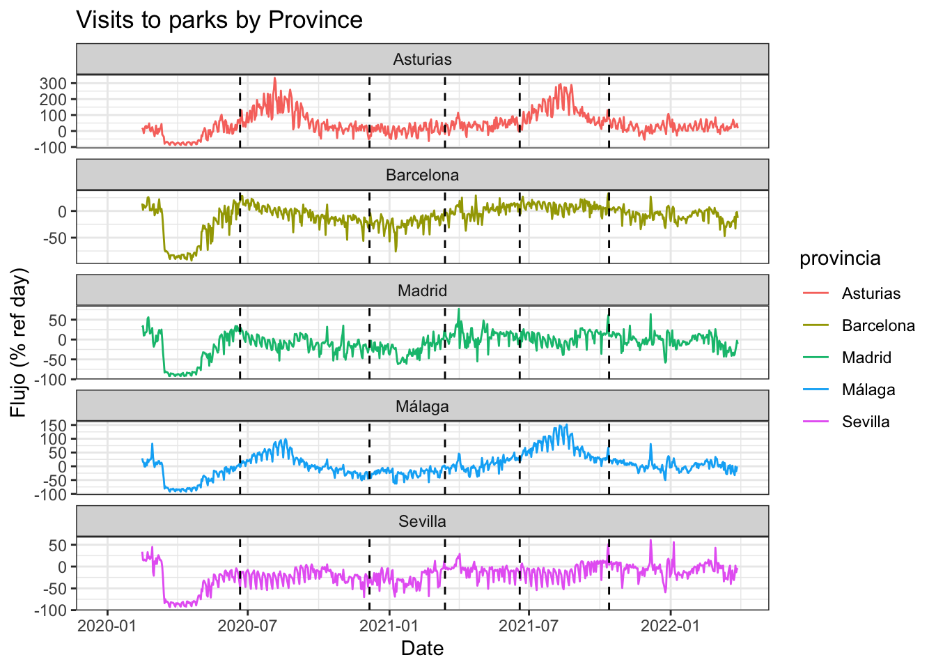
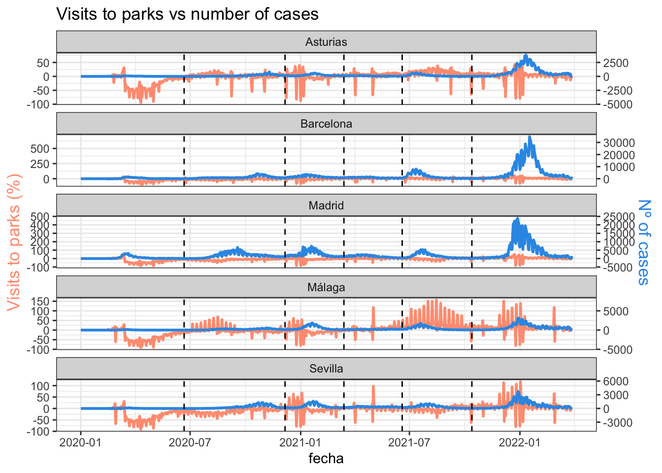
parks

covid_data %>% 
      ggplot(aes(x = fecha)) +
      geom_line(aes(y = mob_parks, color = provincia)) +
      geom_vline(xintercept = as.Date("2020-06-21", format = "%Y-%m-%d"), linetype="dashed") +
      geom_vline(xintercept = as.Date("2020-12-06", format = "%Y-%m-%d"), linetype="dashed") +
      geom_vline(xintercept = as.Date("2021-03-14", format = "%Y-%m-%d"), linetype="dashed") +
      geom_vline(xintercept = as.Date("2021-06-19", format = "%Y-%m-%d"), linetype="dashed") +
      geom_vline(xintercept = as.Date("2021-10-13", format = "%Y-%m-%d"), linetype="dashed") +
      facet_wrap(~provincia, scales = "free_y", ncol=1) +
      theme(legend.position = "top") +
      labs(title="Visits to parks by Province",
           x ="Date", y = "Flujo (% ref day)") +
      theme_bw()

# Value used to transform the data
coeff <- 50

# A few constants for colors
temperatureColor <- "#ff9e81"
priceColor <- rgb(0.2, 0.6, 0.9, 1)

covid_data %>% 
      ggplot(aes(x = fecha)) +
      geom_line( aes(y = mob_grocery_pharmacy), size=1, color=temperatureColor) + 
      geom_line( aes(y = num_casos / coeff), size=1, color=priceColor) +
      geom_vline(xintercept = as.Date("2020-06-21", format = "%Y-%m-%d"), linetype="dashed") +
      geom_vline(xintercept = as.Date("2020-12-06", format = "%Y-%m-%d"), linetype="dashed") +
      geom_vline(xintercept = as.Date("2021-03-14", format = "%Y-%m-%d"), linetype="dashed") +
      geom_vline(xintercept = as.Date("2021-06-19", format = "%Y-%m-%d"), linetype="dashed") +
      geom_vline(xintercept = as.Date("2021-10-13", format = "%Y-%m-%d"), linetype="dashed") +
      scale_y_continuous(
            # Features of the first axis
            name = "Visits to parks (%)",
            # Add a second axis and specify its features
            sec.axis = sec_axis(~.*coeff, name="Nº of cases")
      ) +
      facet_wrap(~provincia, scales = "free_y", ncol=1) +
      theme_bw() +
      theme(
            axis.title.y = element_text(color = temperatureColor, size=13),
            axis.title.y.right = element_text(color = priceColor, size=13)
      ) +
      ggtitle("Visits to parks vs number of cases")

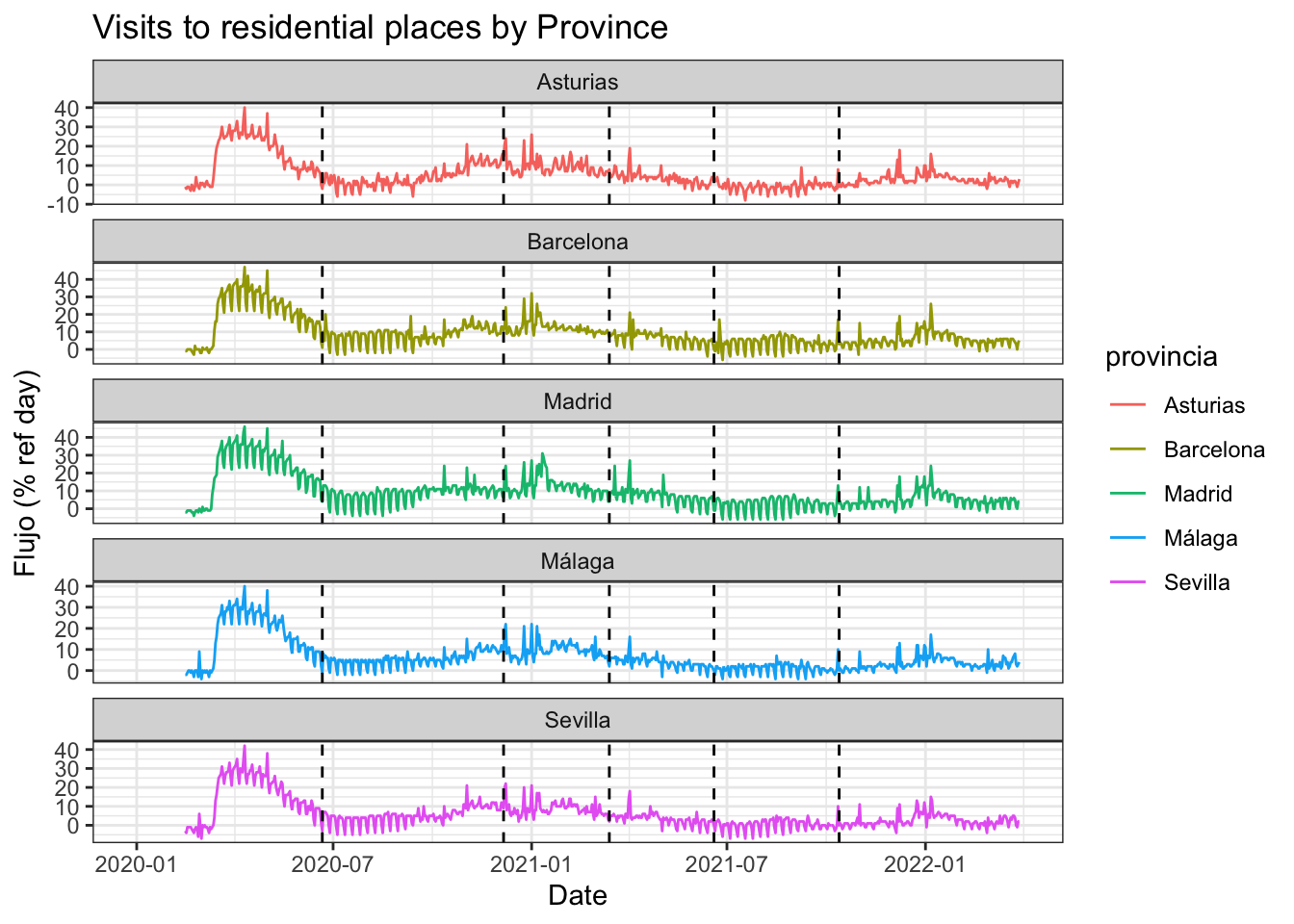
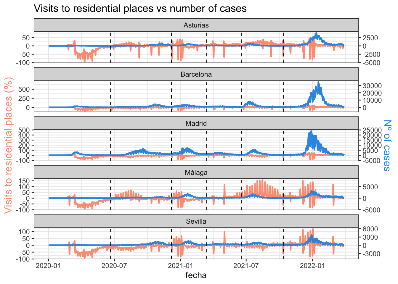
residential

covid_data %>% 
      ggplot(aes(x = fecha)) +
      geom_line(aes(y = mob_residential, color = provincia)) +
      geom_vline(xintercept = as.Date("2020-06-21", format = "%Y-%m-%d"), linetype="dashed") +
      geom_vline(xintercept = as.Date("2020-12-06", format = "%Y-%m-%d"), linetype="dashed") +
      geom_vline(xintercept = as.Date("2021-03-14", format = "%Y-%m-%d"), linetype="dashed") +
      geom_vline(xintercept = as.Date("2021-06-19", format = "%Y-%m-%d"), linetype="dashed") +
      geom_vline(xintercept = as.Date("2021-10-13", format = "%Y-%m-%d"), linetype="dashed") +
      facet_wrap(~provincia, scales = "free_y", ncol=1) +
      theme(legend.position = "top") +
      labs(title="Visits to residential places by Province",
           x ="Date", y = "Flujo (% ref day)") +
      theme_bw()

# Value used to transform the data
coeff <- 50

# A few constants for colors
temperatureColor <- "#ff9e81"
priceColor <- rgb(0.2, 0.6, 0.9, 1)

covid_data %>% 
      ggplot(aes(x = fecha)) +
      geom_line( aes(y = mob_grocery_pharmacy), size=1, color=temperatureColor) + 
      geom_line( aes(y = num_casos / coeff), size=1, color=priceColor) +
      geom_vline(xintercept = as.Date("2020-06-21", format = "%Y-%m-%d"), linetype="dashed") +
      geom_vline(xintercept = as.Date("2020-12-06", format = "%Y-%m-%d"), linetype="dashed") +
      geom_vline(xintercept = as.Date("2021-03-14", format = "%Y-%m-%d"), linetype="dashed") +
      geom_vline(xintercept = as.Date("2021-06-19", format = "%Y-%m-%d"), linetype="dashed") +
      geom_vline(xintercept = as.Date("2021-10-13", format = "%Y-%m-%d"), linetype="dashed") +
      scale_y_continuous(
            # Features of the first axis
            name = "Visits to residential places (%)",
            # Add a second axis and specify its features
            sec.axis = sec_axis(~.*coeff, name="Nº of cases")
      ) +
      facet_wrap(~provincia, scales = "free_y", ncol=1) +
      theme_bw() +
      theme(
            axis.title.y = element_text(color = temperatureColor, size=13),
            axis.title.y.right = element_text(color = priceColor, size=13)
      ) +
      ggtitle("Visits to residential places vs number of cases")

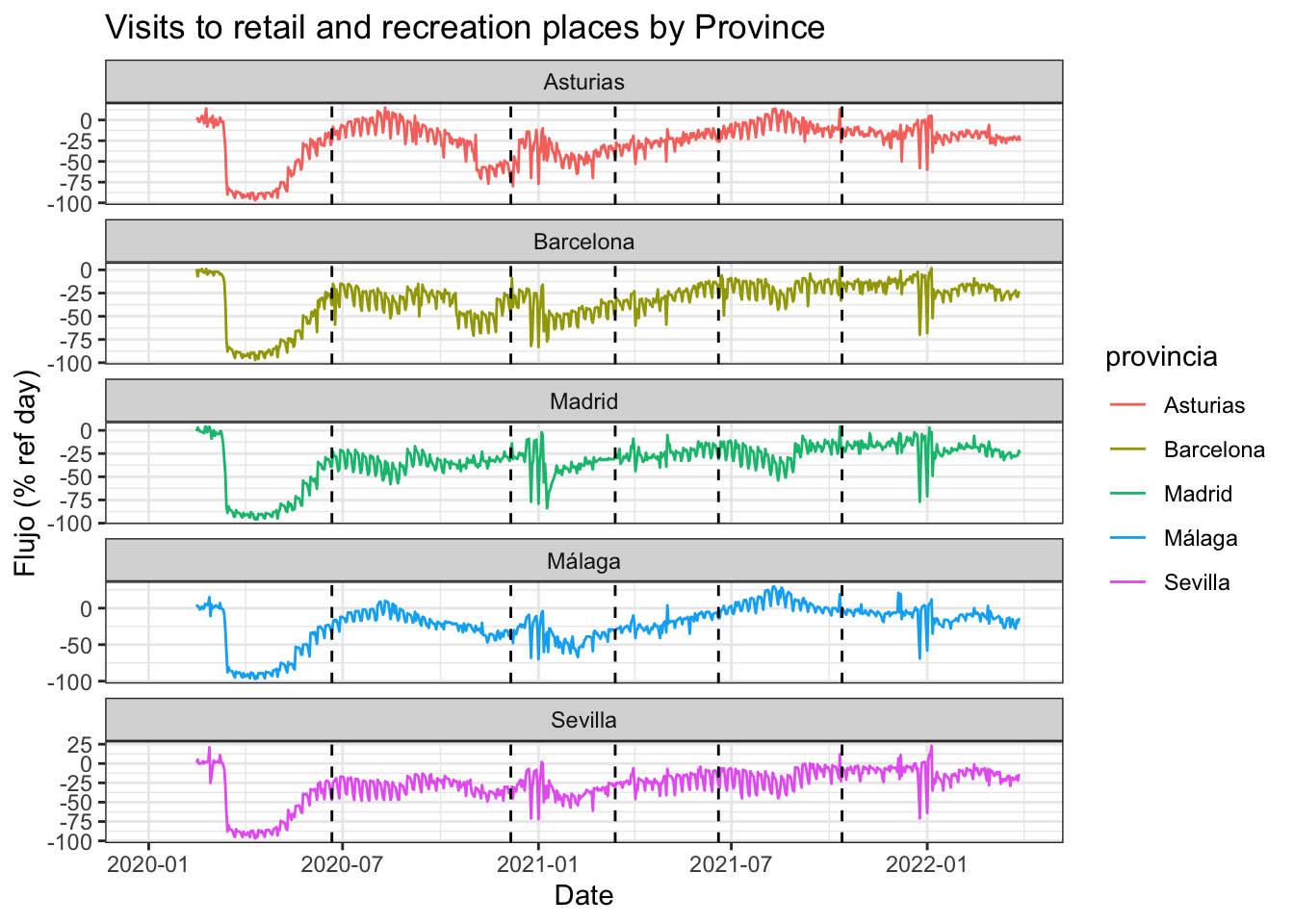
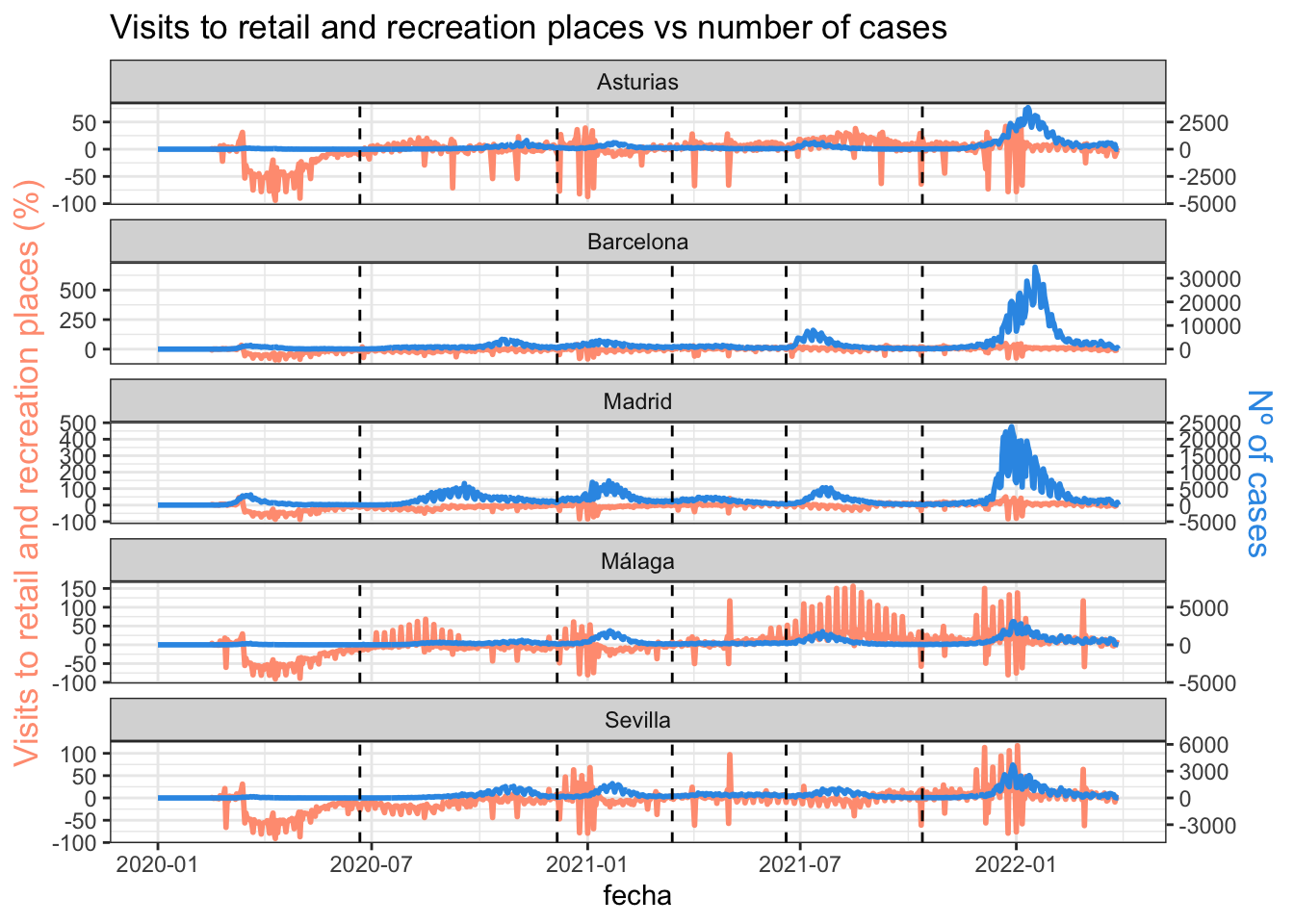
retail and recreation

covid_data %>% 
      ggplot(aes(x = fecha)) +
      geom_line(aes(y = mob_retail_recreation, color = provincia)) +
      geom_vline(xintercept = as.Date("2020-06-21", format = "%Y-%m-%d"), linetype="dashed") +
      geom_vline(xintercept = as.Date("2020-12-06", format = "%Y-%m-%d"), linetype="dashed") +
      geom_vline(xintercept = as.Date("2021-03-14", format = "%Y-%m-%d"), linetype="dashed") +
      geom_vline(xintercept = as.Date("2021-06-19", format = "%Y-%m-%d"), linetype="dashed") +
      geom_vline(xintercept = as.Date("2021-10-13", format = "%Y-%m-%d"), linetype="dashed") +
      facet_wrap(~provincia, scales = "free_y", ncol=1) +
      theme(legend.position = "top") +
      labs(title="Visits to retail and recreation places by Province",
           x ="Date", y = "Flujo (% ref day)") +
      theme_bw()

# Value used to transform the data
coeff <- 50

# A few constants for colors
temperatureColor <- "#ff9e81"
priceColor <- rgb(0.2, 0.6, 0.9, 1)

covid_data %>% 
      ggplot(aes(x = fecha)) +
      geom_line( aes(y = mob_grocery_pharmacy), size=1, color=temperatureColor) + 
      geom_line( aes(y = num_casos / coeff), size=1, color=priceColor) +
      geom_vline(xintercept = as.Date("2020-06-21", format = "%Y-%m-%d"), linetype="dashed") +
      geom_vline(xintercept = as.Date("2020-12-06", format = "%Y-%m-%d"), linetype="dashed") +
      geom_vline(xintercept = as.Date("2021-03-14", format = "%Y-%m-%d"), linetype="dashed") +
      geom_vline(xintercept = as.Date("2021-06-19", format = "%Y-%m-%d"), linetype="dashed") +
      geom_vline(xintercept = as.Date("2021-10-13", format = "%Y-%m-%d"), linetype="dashed") +
      scale_y_continuous(
            # Features of the first axis
            name = "Visits to retail and recreation places (%)",
            # Add a second axis and specify its features
            sec.axis = sec_axis(~.*coeff, name="Nº of cases")
      ) +
      facet_wrap(~provincia, scales = "free_y", ncol=1) +
      theme_bw() +
      theme(
            axis.title.y = element_text(color = temperatureColor, size=13),
            axis.title.y.right = element_text(color = priceColor, size=13)
      ) +
      ggtitle("Visits to retail and recreation places vs number of cases")

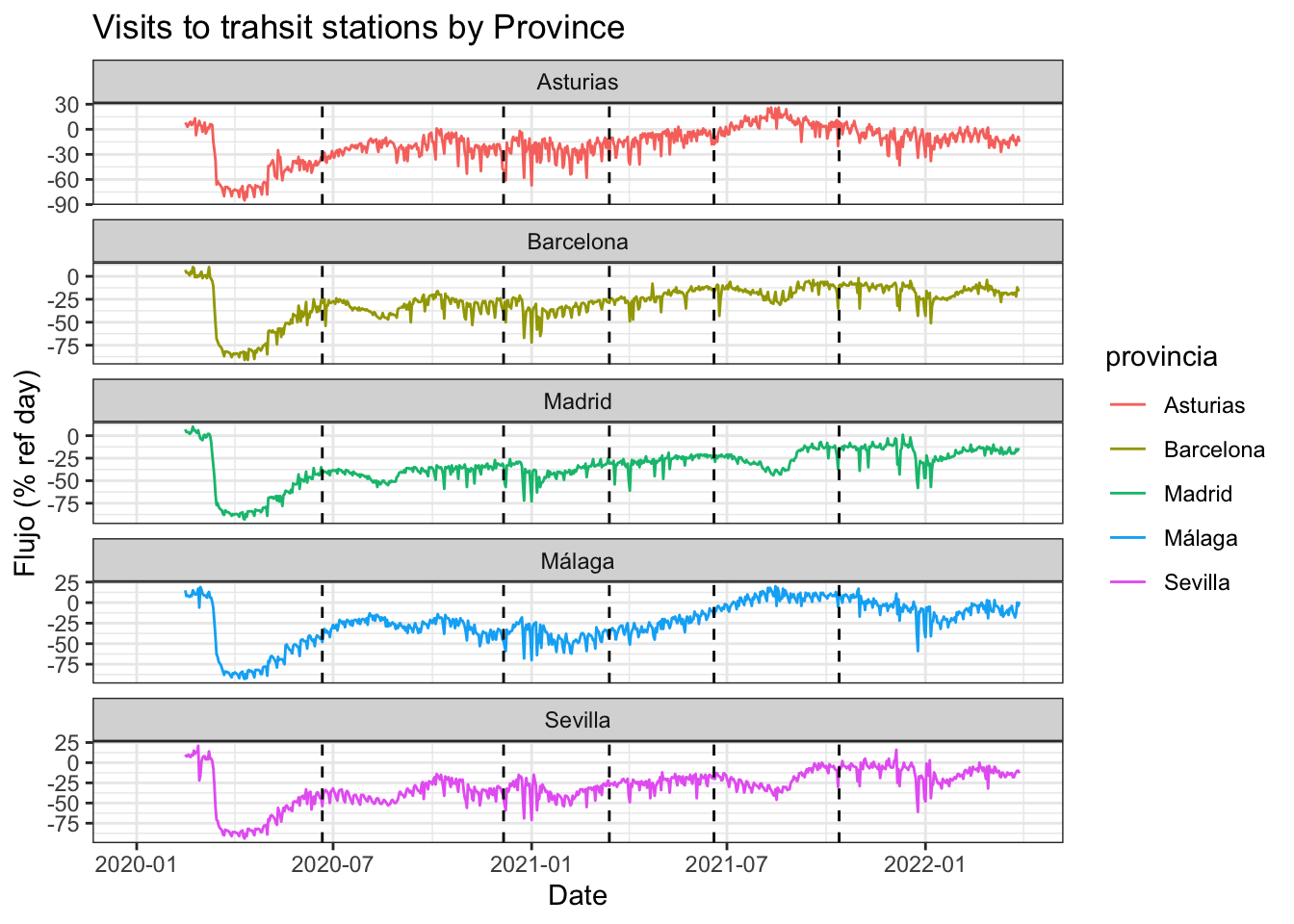
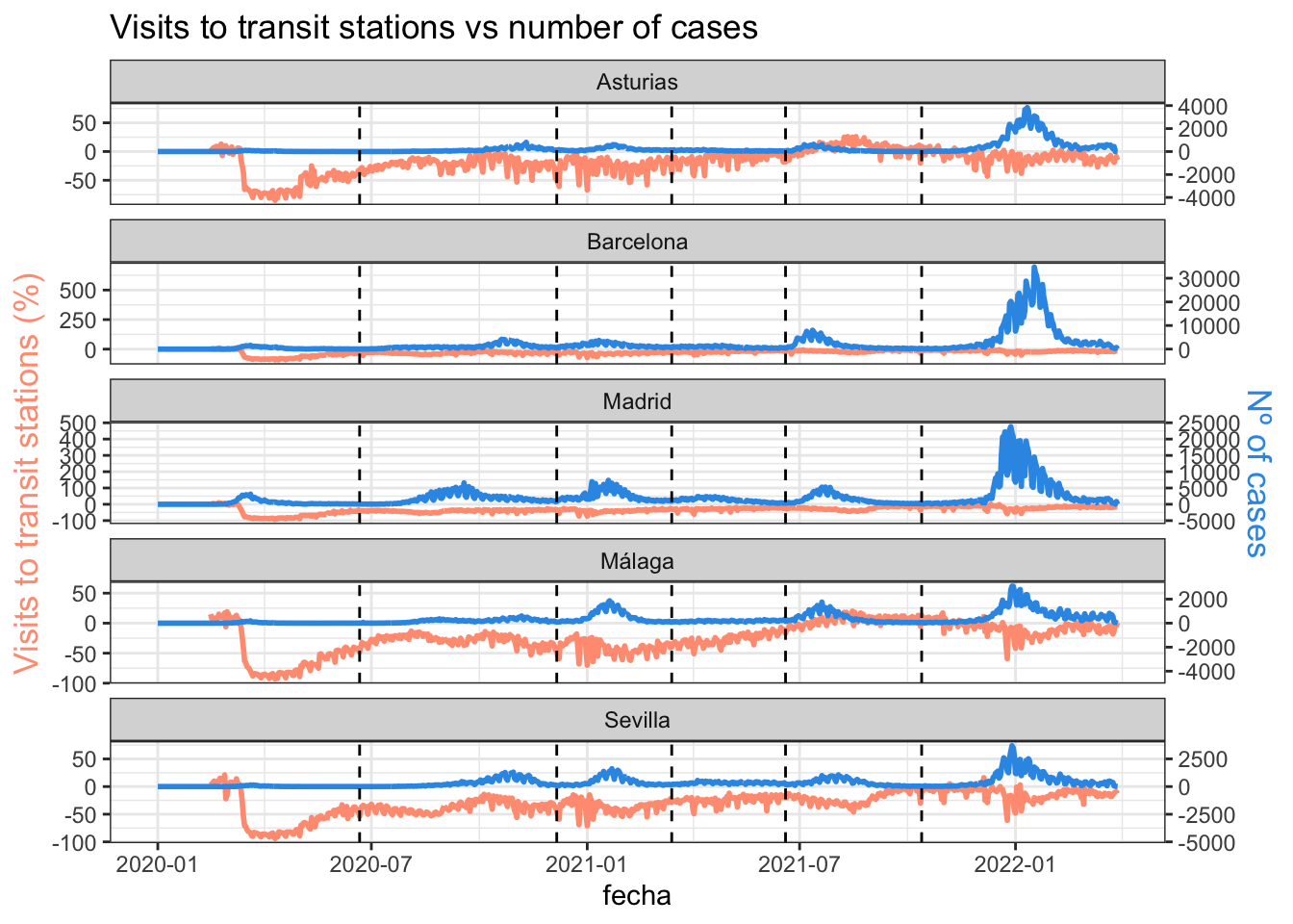
transit stations

covid_data %>% 
      ggplot(aes(x = fecha)) +
      geom_line(aes(y = mob_transit_stations, color = provincia)) +
      geom_vline(xintercept = as.Date("2020-06-21", format = "%Y-%m-%d"), linetype="dashed") +
      geom_vline(xintercept = as.Date("2020-12-06", format = "%Y-%m-%d"), linetype="dashed") +
      geom_vline(xintercept = as.Date("2021-03-14", format = "%Y-%m-%d"), linetype="dashed") +
      geom_vline(xintercept = as.Date("2021-06-19", format = "%Y-%m-%d"), linetype="dashed") +
      geom_vline(xintercept = as.Date("2021-10-13", format = "%Y-%m-%d"), linetype="dashed") +
      facet_wrap(~provincia, scales = "free_y", ncol=1) +
      theme(legend.position = "top") +
      labs(title="Visits to trahsit stations by Province",
           x ="Date", y = "Flujo (% ref day)") +
      theme_bw()

# Value used to transform the data
coeff <- 50

# A few constants for colors
temperatureColor <- "#ff9e81"
priceColor <- rgb(0.2, 0.6, 0.9, 1)

covid_data %>% 
      ggplot(aes(x = fecha)) +
      geom_line( aes(y = mob_transit_stations), size=1, color=temperatureColor) + 
      geom_line( aes(y = num_casos / coeff), size=1, color=priceColor) +
      geom_vline(xintercept = as.Date("2020-06-21", format = "%Y-%m-%d"), linetype="dashed") +
      geom_vline(xintercept = as.Date("2020-12-06", format = "%Y-%m-%d"), linetype="dashed") +
      geom_vline(xintercept = as.Date("2021-03-14", format = "%Y-%m-%d"), linetype="dashed") +
      geom_vline(xintercept = as.Date("2021-06-19", format = "%Y-%m-%d"), linetype="dashed") +
      geom_vline(xintercept = as.Date("2021-10-13", format = "%Y-%m-%d"), linetype="dashed") +
      scale_y_continuous(
            # Features of the first axis
            name = "Visits to transit stations (%)",
            # Add a second axis and specify its features
            sec.axis = sec_axis(~.*coeff, name="Nº of cases")
      ) +
      facet_wrap(~provincia, scales = "free_y", ncol=1) +
      theme_bw() +
      theme(
            axis.title.y = element_text(color = temperatureColor, size=13),
            axis.title.y.right = element_text(color = priceColor, size=13)
      ) +
      ggtitle("Visits to transit stations vs number of cases")

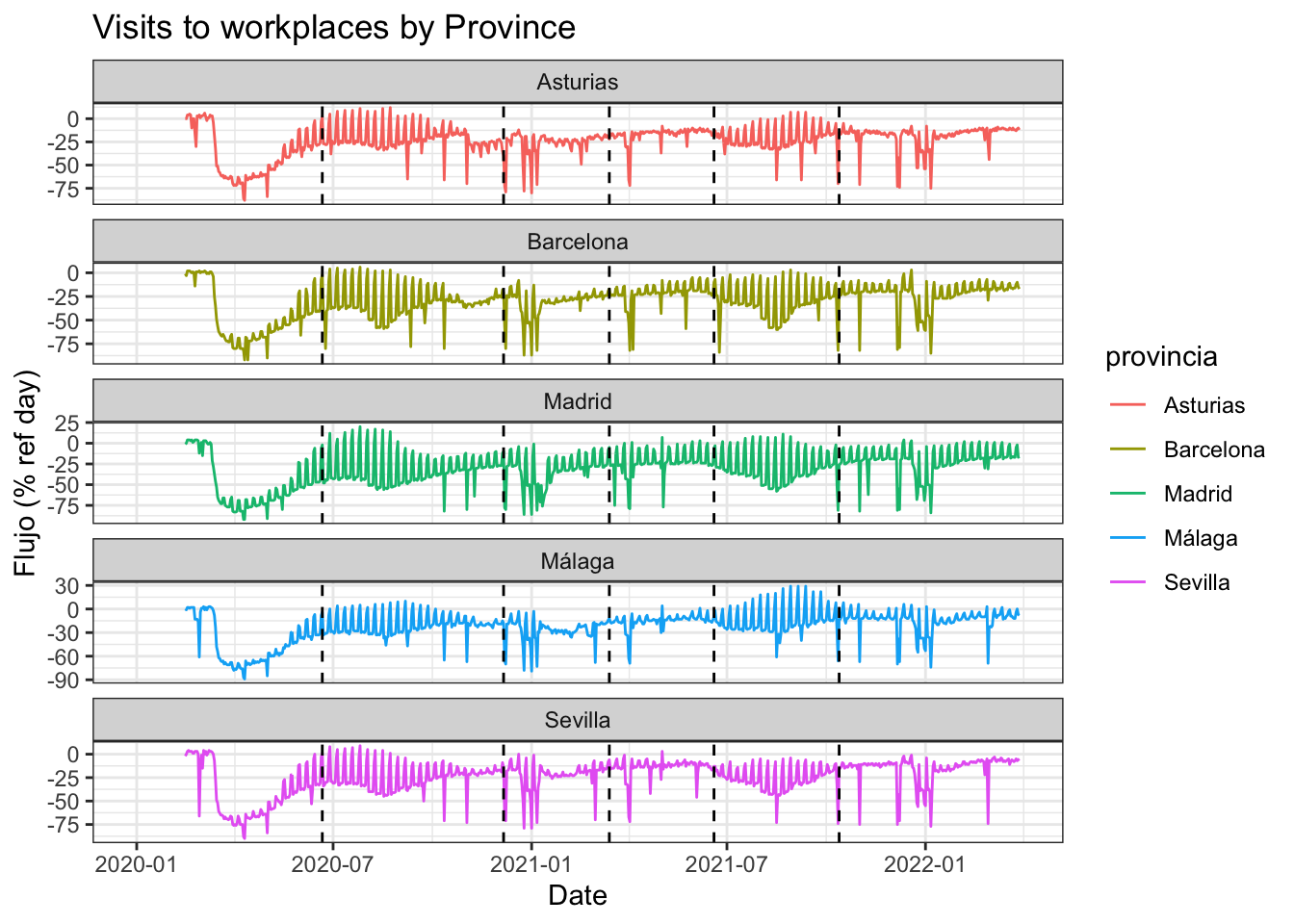
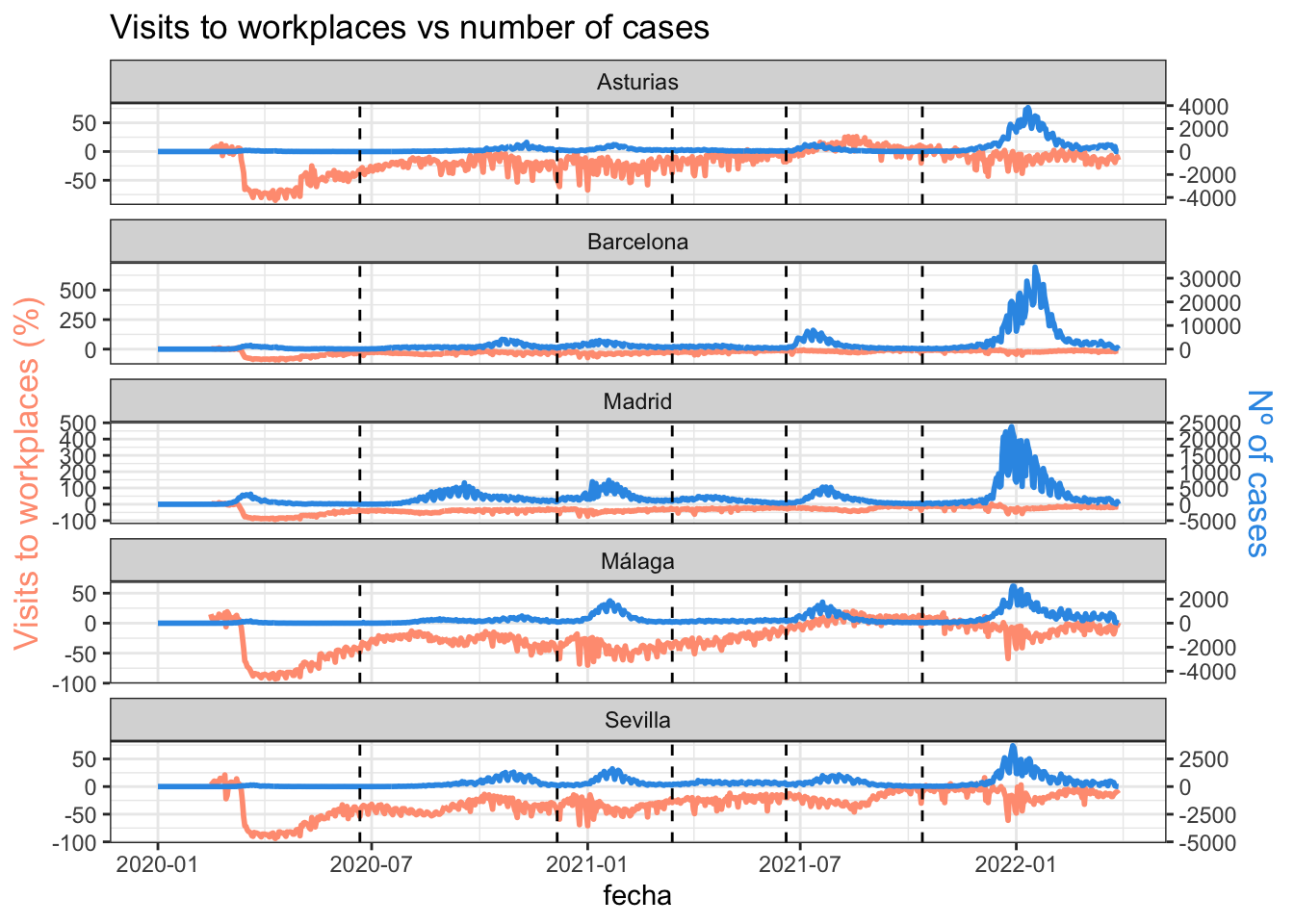
workplaces

covid_data %>% 
      ggplot(aes(x = fecha)) +
      geom_line(aes(y = mob_workplaces, color = provincia)) +
      geom_vline(xintercept = as.Date("2020-06-21", format = "%Y-%m-%d"), linetype="dashed") +
      geom_vline(xintercept = as.Date("2020-12-06", format = "%Y-%m-%d"), linetype="dashed") +
      geom_vline(xintercept = as.Date("2021-03-14", format = "%Y-%m-%d"), linetype="dashed") +
      geom_vline(xintercept = as.Date("2021-06-19", format = "%Y-%m-%d"), linetype="dashed") +
      geom_vline(xintercept = as.Date("2021-10-13", format = "%Y-%m-%d"), linetype="dashed") +
      facet_wrap(~provincia, scales = "free_y", ncol=1) +
      theme(legend.position = "top") +
      labs(title="Visits to workplaces by Province",
           x ="Date", y = "Flujo (% ref day)") +
      theme_bw()

# Value used to transform the data
coeff <- 50

# A few constants for colors
temperatureColor <- "#ff9e81"
priceColor <- rgb(0.2, 0.6, 0.9, 1)

covid_data %>% 
      ggplot(aes(x = fecha)) +
      geom_line( aes(y = mob_transit_stations), size=1, color=temperatureColor) + 
      geom_line( aes(y = num_casos / coeff), size=1, color=priceColor) +
      geom_vline(xintercept = as.Date("2020-06-21", format = "%Y-%m-%d"), linetype="dashed") +
      geom_vline(xintercept = as.Date("2020-12-06", format = "%Y-%m-%d"), linetype="dashed") +
      geom_vline(xintercept = as.Date("2021-03-14", format = "%Y-%m-%d"), linetype="dashed") +
      geom_vline(xintercept = as.Date("2021-06-19", format = "%Y-%m-%d"), linetype="dashed") +
      geom_vline(xintercept = as.Date("2021-10-13", format = "%Y-%m-%d"), linetype="dashed") +
      scale_y_continuous(
            # Features of the first axis
            name = "Visits to workplaces (%)",
            # Add a second axis and specify its features
            sec.axis = sec_axis(~.*coeff, name="Nº of cases")
      ) +
      facet_wrap(~provincia, scales = "free_y", ncol=1) +
      theme_bw() +
      theme(
            axis.title.y = element_text(color = temperatureColor, size=13),
            axis.title.y.right = element_text(color = priceColor, size=13)
      ) +
      ggtitle("Visits to workplaces vs number of cases")

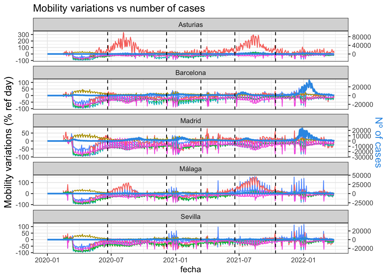
Google mobility vs cases

# Value used to transform the data
coeff <- 300

# A few constants for colors
priceColor <- rgb(0.2, 0.6, 0.9, 1)

p <- covid_data %>% 
      ggplot(aes(x = fecha)) +
      geom_line(aes(x = fecha, y = mob_grocery_pharmacy, color = "red")) +
      geom_line(aes(x = fecha, y = mob_parks, color = "black")) +
      geom_line(aes(x = fecha, y = mob_residential, color = "blue")) +
      geom_line(aes(x = fecha, y = mob_retail_recreation, color = "green")) +
      geom_line(aes(x = fecha, y = mob_transit_stations, color = "brown")) +
      geom_line(aes(x = fecha, y = mob_workplaces, color = "yellow")) +
      geom_line( aes(y = num_casos / coeff), size=1, color=priceColor) +
      geom_vline(xintercept = as.Date("2020-06-21", format = "%Y-%m-%d"), linetype="dashed") +
      geom_vline(xintercept = as.Date("2020-12-06", format = "%Y-%m-%d"), linetype="dashed") +
      geom_vline(xintercept = as.Date("2021-03-14", format = "%Y-%m-%d"), linetype="dashed") +
      geom_vline(xintercept = as.Date("2021-06-19", format = "%Y-%m-%d"), linetype="dashed") +
      geom_vline(xintercept = as.Date("2021-10-13", format = "%Y-%m-%d"), linetype="dashed") +
      scale_y_continuous(
            # Features of the first axis
            name = "Mobility variations (% ref day)",
            # Add a second axis and specify its features
            sec.axis = sec_axis(~.*coeff, name="Nº of cases")
      ) +
      facet_wrap(~provincia, scales = "free_y", ncol=1) +
      theme_bw() +
      theme(
            axis.title.y = element_text(size=13),
            axis.title.y.right = element_text(color = priceColor, size=13),
            legend.position = "none") +
      ggtitle("Mobility variations vs number of cases")

p

# ggplotly(p) # To make the graph interactive

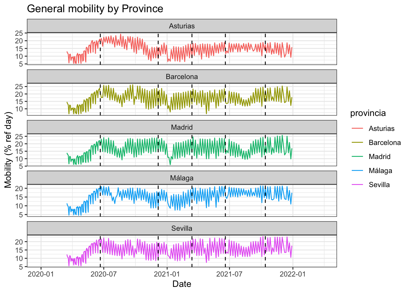
General mobility (INE study zones)

covid_data %>% 
      ggplot(aes(x = fecha)) +
      geom_line(aes(y = mob_flujo, color = provincia)) +
      geom_vline(xintercept = as.Date("2020-06-21", format = "%Y-%m-%d"), linetype="dashed") +
      geom_vline(xintercept = as.Date("2020-12-06", format = "%Y-%m-%d"), linetype="dashed") +
      geom_vline(xintercept = as.Date("2021-03-14", format = "%Y-%m-%d"), linetype="dashed") +
      geom_vline(xintercept = as.Date("2021-06-19", format = "%Y-%m-%d"), linetype="dashed") +
      geom_vline(xintercept = as.Date("2021-10-13", format = "%Y-%m-%d"), linetype="dashed") +
      facet_wrap(~provincia, scales = "free_y", ncol=1) +
      theme(legend.position = "top") +
      labs(title="General mobility by Province",
           x ="Date", y = "Mobility (% ref day)") +
      theme_bw()

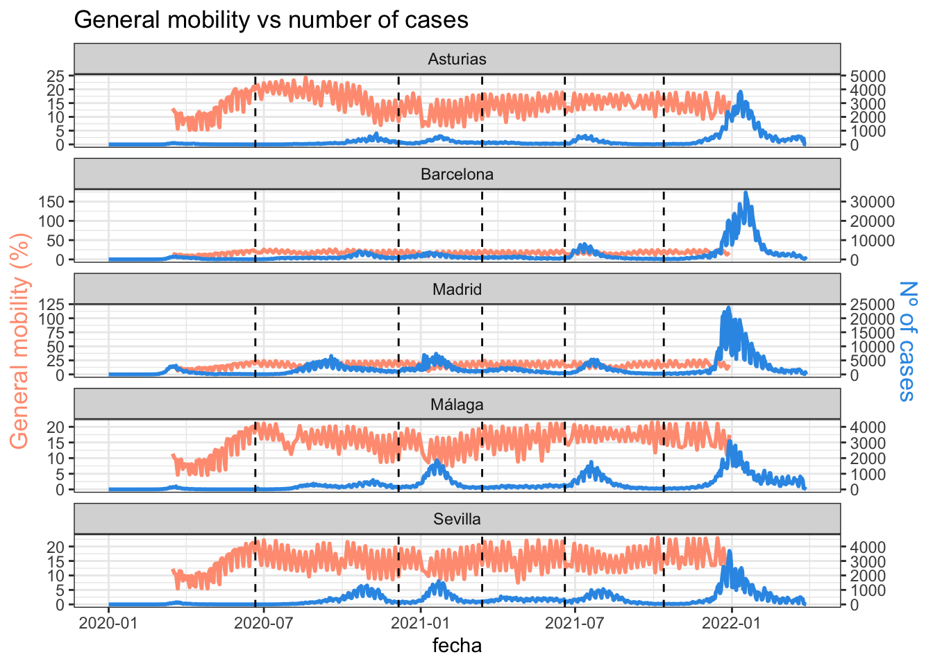
# Value used to transform the data
coeff <- 200

# A few constants for colors
temperatureColor <- "#ff9e81"
priceColor <- rgb(0.2, 0.6, 0.9, 1)

covid_data %>% 
      ggplot(aes(x = fecha)) +
      geom_line( aes(y = mob_flujo), size=1, color=temperatureColor) + 
      geom_line( aes(y = num_casos / coeff), size=1, color=priceColor) +
      geom_vline(xintercept = as.Date("2020-06-21", format = "%Y-%m-%d"), linetype="dashed") +
      geom_vline(xintercept = as.Date("2020-12-06", format = "%Y-%m-%d"), linetype="dashed") +
      geom_vline(xintercept = as.Date("2021-03-14", format = "%Y-%m-%d"), linetype="dashed") +
      geom_vline(xintercept = as.Date("2021-06-19", format = "%Y-%m-%d"), linetype="dashed") +
      geom_vline(xintercept = as.Date("2021-10-13", format = "%Y-%m-%d"), linetype="dashed") +
      scale_y_continuous(
            # Features of the first axis
            name = "General mobility (%)",
            # Add a second axis and specify its features
            sec.axis = sec_axis(~.*coeff, name="Nº of cases")
      ) +
      facet_wrap(~provincia, scales = "free_y", ncol=1) +
      theme_bw() +
      theme(
            axis.title.y = element_text(color = temperatureColor, size=13),
            axis.title.y.right = element_text(color = priceColor, size=13)
      ) +
      ggtitle("General mobility vs number of cases")

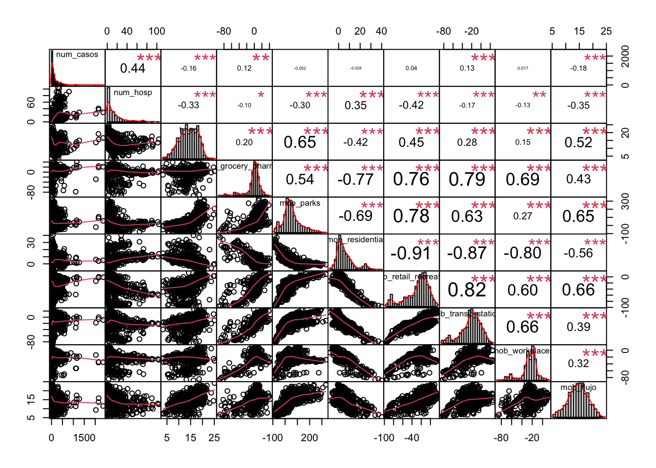
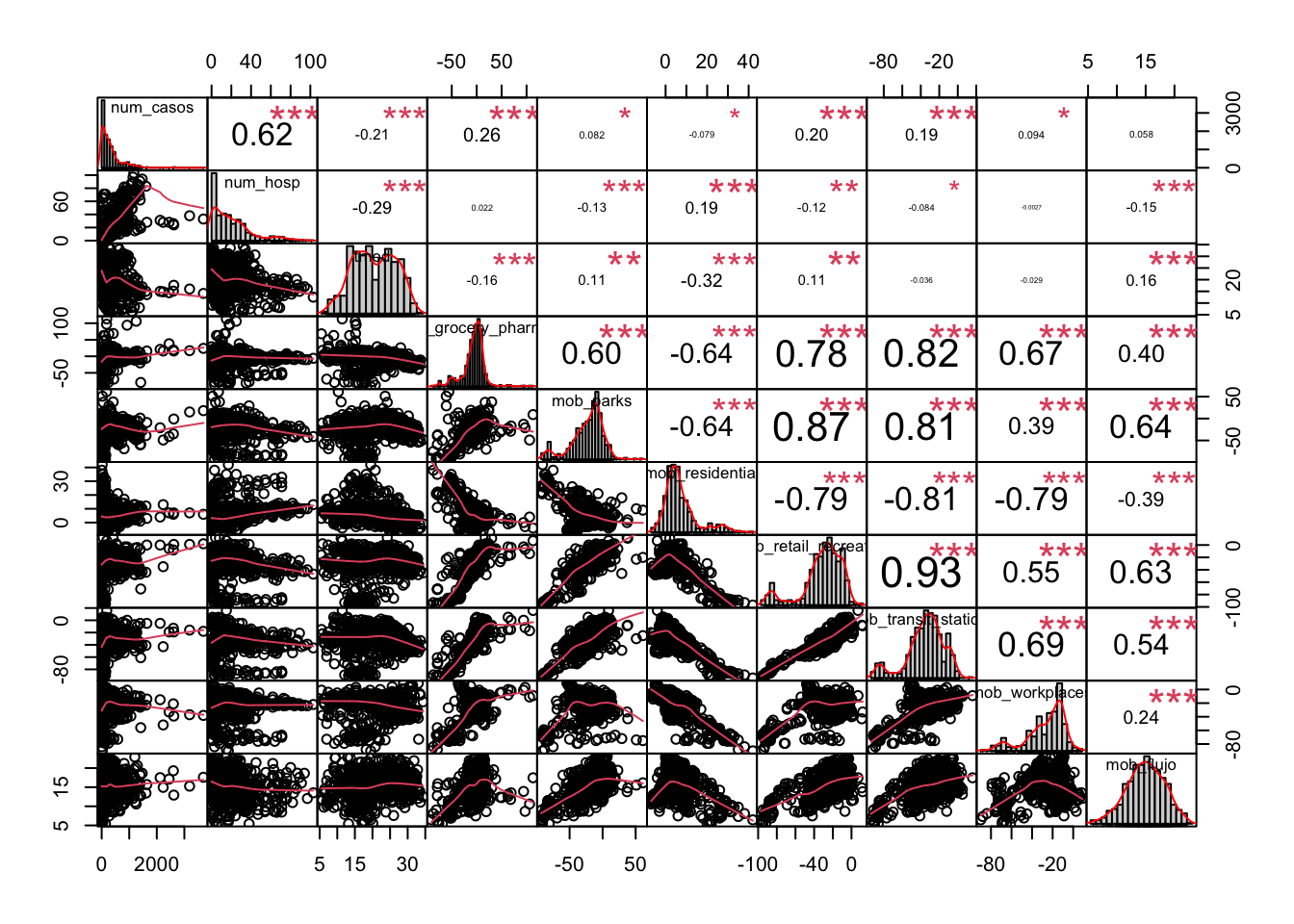
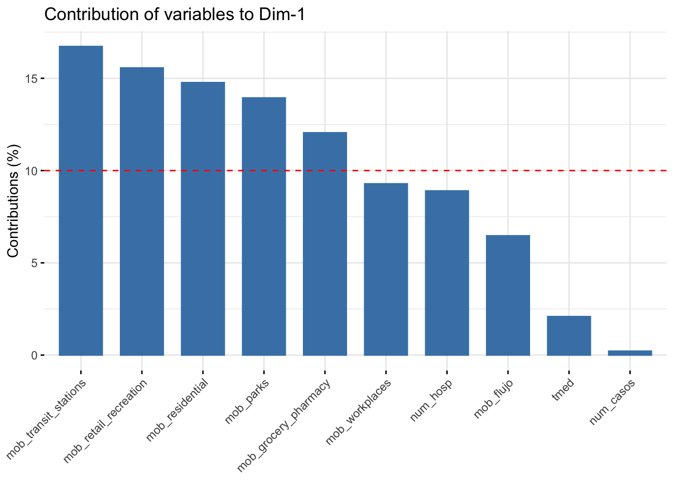
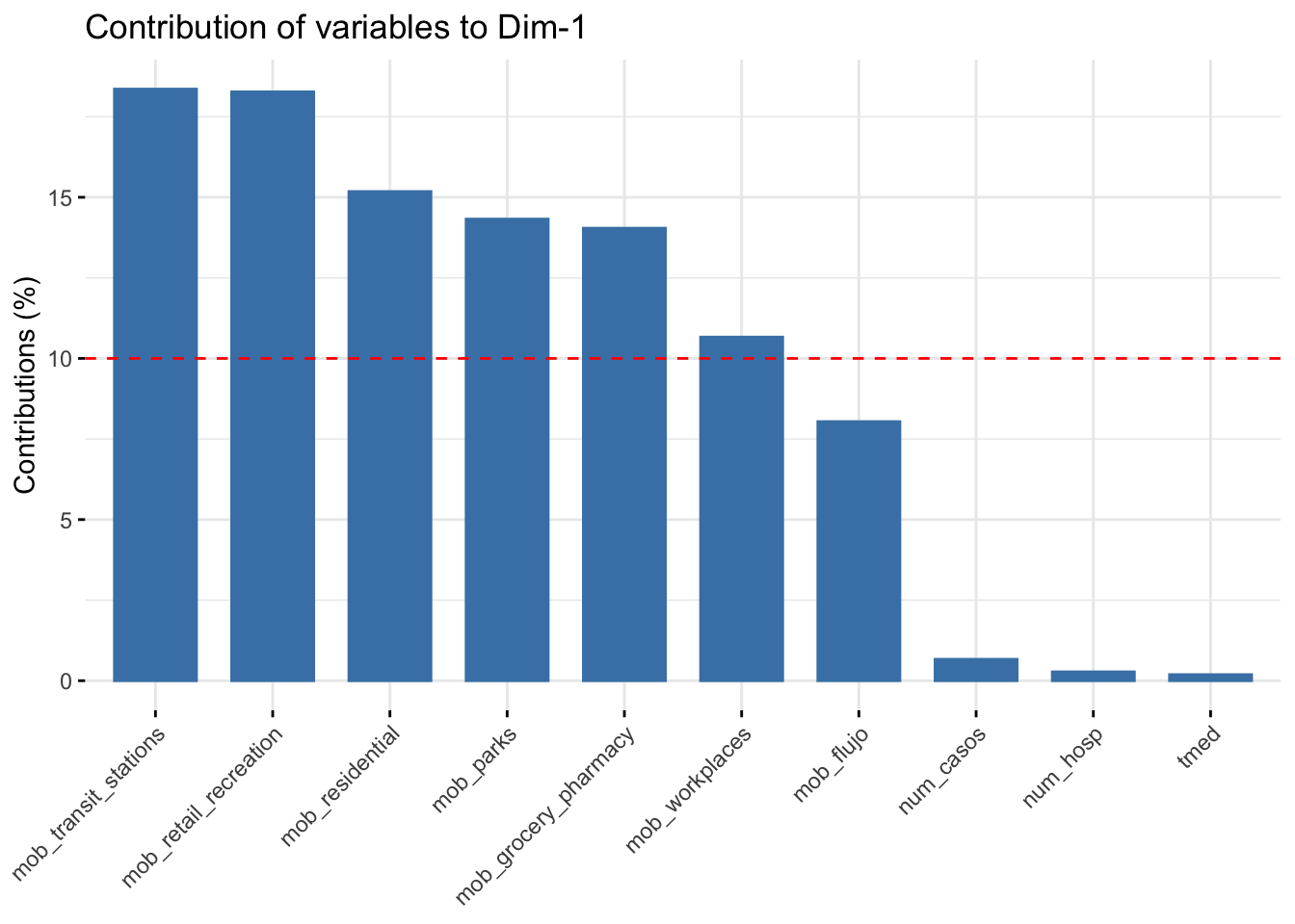
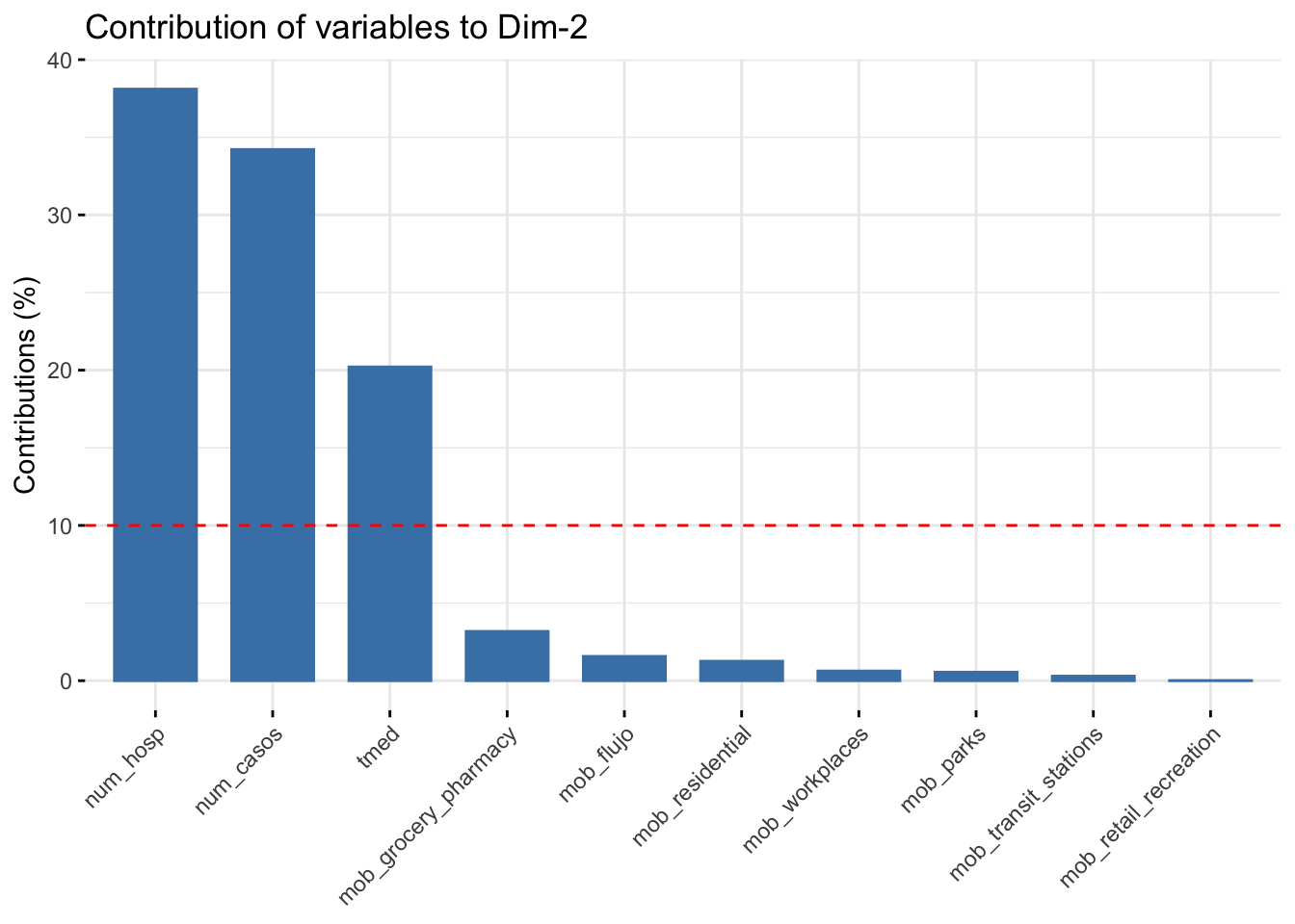
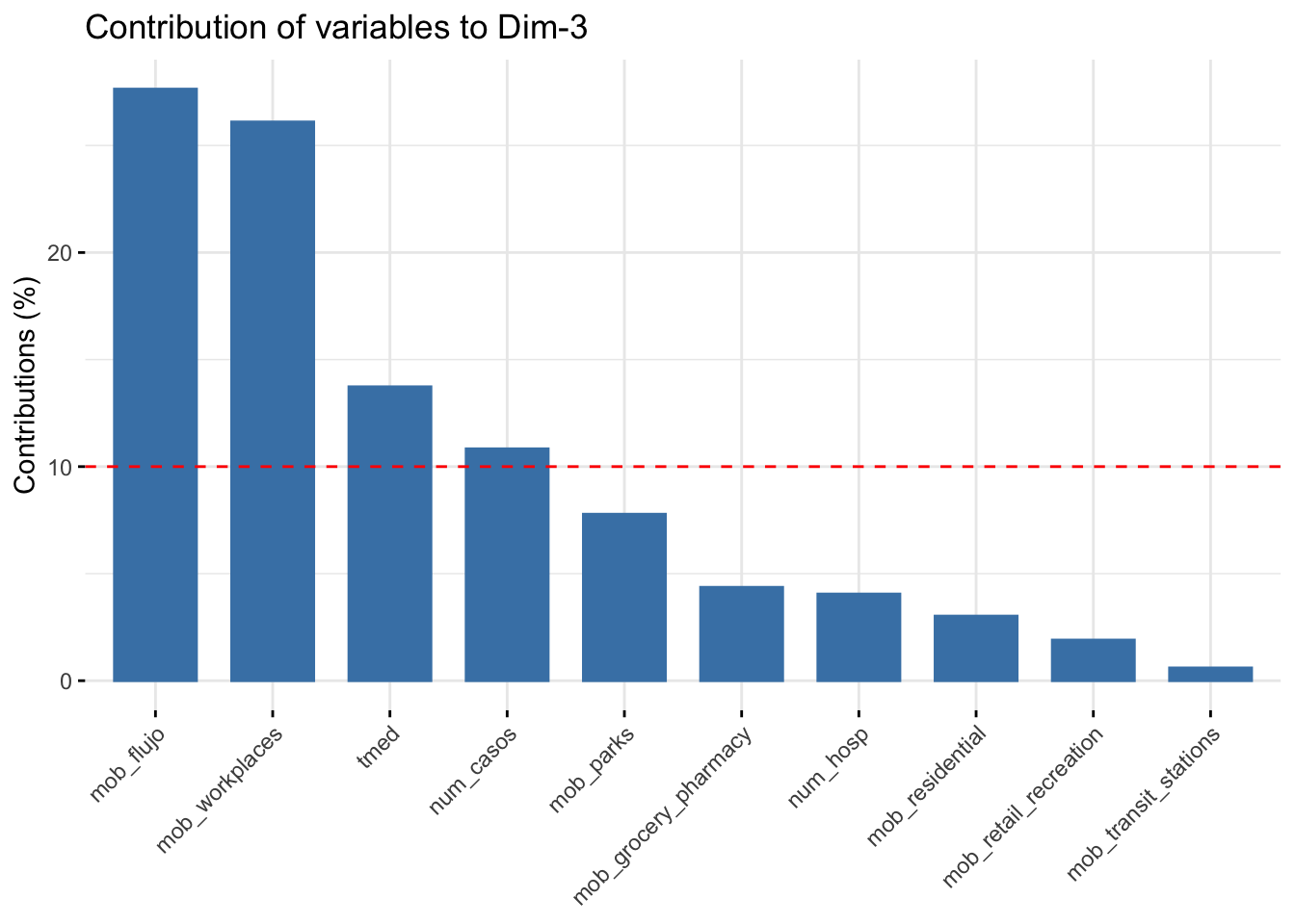
Correlations

From previous visual analysis, we will focus our attention in the following variables:

• num_casos
• num_hosp
• tmed
• mob_grocery_pharmacy
• mob_parks
• mob_residential
• mob_retail_recreation
• mob_transit_stations
• mob_workplaces
• mob_flujo

Asturias

data_asturias <- covid_data %>% 
      filter(provincia == "Asturias") %>% 
      select(num_casos, num_hosp, tmed, mob_grocery_pharmacy, mob_parks, mob_residential, mob_retail_recreation, mob_transit_stations, mob_workplaces, mob_flujo) %>% 
      drop_na()

chart.Correlation(data_asturias, histogram=TRUE, pch=19)

Barcelona

data_barcelona <- covid_data %>% 
      filter(provincia == "Barcelona") %>% 
      select(num_casos, num_hosp, tmed, mob_grocery_pharmacy, mob_parks, mob_residential, mob_retail_recreation, mob_transit_stations, mob_workplaces, mob_flujo) %>% 
      drop_na()

chart.Correlation(data_barcelona, histogram=TRUE, pch=19)

Madrid

data_madrid <- covid_data %>% 
      filter(provincia == "Madrid") %>% 
      select(num_casos, num_hosp, tmed, mob_grocery_pharmacy, mob_parks, mob_residential, mob_retail_recreation, mob_transit_stations, mob_workplaces, mob_flujo) %>% 
      drop_na()

chart.Correlation(data_madrid, histogram=TRUE, pch=19)

Málaga

data_malaga <- covid_data %>% 
      filter(provincia == "Málaga") %>% 
      select(num_casos, num_hosp, tmed, mob_grocery_pharmacy, mob_parks, mob_residential, mob_retail_recreation, mob_transit_stations, mob_workplaces, mob_flujo) %>% 
      drop_na()

chart.Correlation(data_malaga, histogram=TRUE, pch=19)

Sevilla

data_sevilla <- covid_data %>% 
      filter(provincia == "Sevilla") %>% 
      select(num_casos, num_hosp, tmed, mob_grocery_pharmacy, mob_parks, mob_residential, mob_retail_recreation, mob_transit_stations, mob_workplaces, mob_flujo) %>% 
      drop_na()

chart.Correlation(data_sevilla, histogram=TRUE, pch=19)

PCA Analysis

Asturias

pca_asturias <- prcomp(data_asturias, scale = TRUE)
pca_asturias

Standard deviations (1, .., p=10):
 [1] 2.3059001 1.3226315 1.0074444 0.7450691 0.6877792 0.6487611 0.4720477
 [8] 0.3739715 0.2771883 0.1730609

Rotation (n x k) = (10 x 10):
                              PC1         PC2         PC3          PC4
num_casos              0.01450525  0.54489655 -0.51479322 -0.504451200
num_hosp               0.17409928  0.48500003 -0.37126430  0.690242359
tmed                  -0.23699079 -0.37307749 -0.45271462  0.180603004
mob_grocery_pharmacy  -0.35143243  0.28170300  0.11727970  0.126424273
mob_parks             -0.35125168 -0.17159147 -0.38598591 -0.009257317
mob_residential        0.41391323 -0.10601760 -0.11975556  0.054838852
mob_retail_recreation -0.41354502  0.01666112 -0.02232460 -0.211710973
mob_transit_stations  -0.37337796  0.24040335  0.05162636 -0.093305650
mob_workplaces        -0.30382828  0.27686746  0.41962650  0.287377141
mob_flujo             -0.30391699 -0.27186212 -0.18939142  0.285110210
                               PC5         PC6         PC7          PC8
num_casos              0.007707022 -0.39838507  0.05559284 -0.036405423
num_hosp               0.027047134  0.16172768 -0.17598501  0.008142094
tmed                  -0.642379737 -0.18881088  0.25498953  0.215754643
mob_grocery_pharmacy   0.158062302  0.20143454  0.82468490 -0.057629741
mob_parks              0.059354627  0.41906472 -0.19336176 -0.582750644
mob_residential        0.136078986  0.07056199  0.29416933  0.118367813
mob_retail_recreation  0.151941611  0.03708067 -0.07486246 -0.043270088
mob_transit_stations  -0.084870133  0.37541715 -0.26001692  0.682427007
mob_workplaces        -0.299536399 -0.45193891 -0.13878486 -0.273372087
mob_flujo              0.647705124 -0.46016524 -0.06644608  0.229818685
                              PC9         PC10
num_casos             -0.14106177 -0.017603053
num_hosp               0.24578351  0.043113614
tmed                   0.08461699 -0.007038261
mob_grocery_pharmacy  -0.06341817  0.119971853
mob_parks             -0.34415326 -0.153430890
mob_residential       -0.13120769 -0.811682780
mob_retail_recreation  0.79014122 -0.356541626
mob_transit_stations  -0.28731159 -0.165588538
mob_workplaces        -0.19739302 -0.381355987
mob_flujo             -0.16437188  0.032321955

summary(pca_asturias)

Importance of components:
                          PC1    PC2    PC3     PC4    PC5     PC6     PC7
Standard deviation     2.3059 1.3226 1.0074 0.74507 0.6878 0.64876 0.47205
Proportion of Variance 0.5317 0.1749 0.1015 0.05551 0.0473 0.04209 0.02228
Cumulative Proportion  0.5317 0.7067 0.8082 0.86366 0.9110 0.95305 0.97534
                           PC8     PC9   PC10
Standard deviation     0.37397 0.27719 0.1731
Proportion of Variance 0.01399 0.00768 0.0030
Cumulative Proportion  0.98932 0.99700 1.0000

fviz_contrib(pca_asturias, choice = "var", axes = 1)

fviz_contrib(pca_asturias, choice = "var", axes = 2)

fviz_contrib(pca_asturias, choice = "var", axes = 3)

Barcelona

pca_barcelona <- prcomp(data_barcelona, scale = TRUE)
pca_barcelona

Standard deviations (1, .., p=10):
 [1] 2.3500494 1.1639307 1.0203223 0.8907862 0.7077661 0.5991284 0.4632802
 [8] 0.3564024 0.2192014 0.1959267

Rotation (n x k) = (10 x 10):
                              PC1          PC2         PC3          PC4
num_casos             -0.04635023  0.570768442  0.53457698 -0.492988960
num_hosp               0.29831071  0.284686532  0.09436374 -0.034833462
tmed                  -0.14449540 -0.626623503  0.30664954 -0.452229899
mob_grocery_pharmacy  -0.34713681  0.337004339  0.02002121  0.151561449
mob_parks             -0.37335503 -0.193131167  0.18530647 -0.084926570
mob_residential        0.38430706  0.007416082  0.24886368  0.259624192
mob_retail_recreation -0.39452627  0.063798737  0.18765830  0.069063116
mob_transit_stations  -0.40897022  0.127987718 -0.07637794  0.004222074
mob_workplaces        -0.30468032  0.155504866 -0.55283186 -0.129464416
mob_flujo             -0.25427521 -0.070430679  0.40981000  0.657343094
                              PC5         PC6         PC7          PC8
num_casos              0.19339495  0.32350158 -0.00629119  0.030606330
num_hosp              -0.85463757 -0.17161237 -0.22533531  0.094962761
tmed                  -0.33093566  0.09231281  0.39889639 -0.006104091
mob_grocery_pharmacy  -0.08132938 -0.39493763  0.65121038  0.249245145
mob_parks              0.08850418 -0.27365929 -0.49626105  0.644319123
mob_residential        0.14832065 -0.12032335  0.28408811  0.321039366
mob_retail_recreation -0.07064019 -0.29899673 -0.08915710 -0.584504519
mob_transit_stations  -0.06330964 -0.11946594 -0.12154825 -0.072176343
mob_workplaces        -0.20404108  0.48022022  0.12291337  0.248375683
mob_flujo             -0.18867227  0.52701879 -0.03434211  0.033557108
                               PC9        PC10
num_casos             -0.002320569  0.01509282
num_hosp               0.003777920  0.01349170
tmed                  -0.092334422  0.04687160
mob_grocery_pharmacy   0.134095696 -0.27528609
mob_parks              0.182419504  0.06583257
mob_residential       -0.196882515  0.68110459
mob_retail_recreation  0.329721528  0.49758768
mob_transit_stations  -0.875118234  0.08009707
mob_workplaces         0.163742743  0.42982550
mob_flujo              0.008575829 -0.12089009

summary(pca_barcelona)

Importance of components:
                          PC1    PC2    PC3     PC4     PC5    PC6     PC7
Standard deviation     2.3500 1.1639 1.0203 0.89079 0.70777 0.5991 0.46328
Proportion of Variance 0.5523 0.1355 0.1041 0.07935 0.05009 0.0359 0.02146
Cumulative Proportion  0.5523 0.6877 0.7919 0.87120 0.92130 0.9572 0.97865
                          PC8    PC9    PC10
Standard deviation     0.3564 0.2192 0.19593
Proportion of Variance 0.0127 0.0048 0.00384
Cumulative Proportion  0.9914 0.9962 1.00000

fviz_contrib(pca_barcelona, choice = "var", axes = 1)

fviz_contrib(pca_barcelona, choice = "var", axes = 2)

fviz_contrib(pca_barcelona, choice = "var", axes = 3)

Madrid

pca_madrid <- prcomp(data_madrid, scale = TRUE)
pca_madrid

Standard deviations (1, .., p=10):
 [1] 2.2848571 1.2225837 1.0319540 0.9173293 0.7538326 0.6158312 0.4456798
 [8] 0.3743592 0.2529196 0.1674507

Rotation (n x k) = (10 x 10):
                              PC1        PC2         PC3         PC4
num_casos             -0.01423162  0.5854425  0.06882652 -0.70306268
num_hosp               0.27600601  0.3157810  0.06783645 -0.12215647
tmed                  -0.06116377 -0.6156756 -0.18467058 -0.61357270
mob_grocery_pharmacy  -0.37932123  0.2832513 -0.04936637  0.05230846
mob_parks             -0.36244379 -0.1197542 -0.28139926 -0.13467682
mob_residential        0.37894331  0.1601416 -0.35460347  0.16002713
mob_retail_recreation -0.40910449  0.1516826 -0.11182971 -0.05493973
mob_transit_stations  -0.41730212  0.1056251  0.08377947  0.08242167
mob_workplaces        -0.30627182 -0.0855751  0.59690452  0.12801981
mob_flujo             -0.25635724  0.1295295 -0.61104157  0.20402385
                              PC5         PC6         PC7          PC8
num_casos              0.24552109 -0.26345562  0.15328157 -0.040875827
num_hosp              -0.83725304  0.30701841  0.09072498 -0.004431129
tmed                  -0.25238790 -0.12186856 -0.28247772 -0.112257979
mob_grocery_pharmacy  -0.04343098  0.12704931 -0.62858714 -0.502353135
mob_parks              0.09156988  0.51766298  0.59572642 -0.336804286
mob_residential        0.14343571  0.06769104 -0.09643941 -0.444183532
mob_retail_recreation -0.03488279  0.25135710 -0.16413678  0.371254042
mob_transit_stations  -0.05857713  0.08498906 -0.07417955  0.302309594
mob_workplaces        -0.20465773 -0.32418049  0.23925417 -0.438932910
mob_flujo             -0.31248859 -0.59773222  0.19870007  0.027020637
                              PC9        PC10
num_casos              0.04735181 -0.03037372
num_hosp               0.02858333  0.01607570
tmed                   0.09549151 -0.16297889
mob_grocery_pharmacy  -0.02709125  0.32321617
mob_parks              0.03477439  0.10523166
mob_residential        0.17235888 -0.64648380
mob_retail_recreation -0.54936170 -0.51296756
mob_transit_stations   0.79984701 -0.23148779
mob_workplaces        -0.11524111 -0.34062802
mob_flujo             -0.03656999  0.07761072

summary(pca_madrid)

Importance of components:
                          PC1    PC2    PC3     PC4     PC5     PC6     PC7
Standard deviation     2.2849 1.2226 1.0320 0.91733 0.75383 0.61583 0.44568
Proportion of Variance 0.5221 0.1495 0.1065 0.08415 0.05683 0.03792 0.01986
Cumulative Proportion  0.5221 0.6715 0.7780 0.86217 0.91900 0.95692 0.97678
                           PC8    PC9   PC10
Standard deviation     0.37436 0.2529 0.1675
Proportion of Variance 0.01401 0.0064 0.0028
Cumulative Proportion  0.99080 0.9972 1.0000

fviz_contrib(pca_madrid, choice = "var", axes = 1)

fviz_contrib(pca_madrid, choice = "var", axes = 2)

fviz_contrib(pca_madrid, choice = "var", axes = 3)

Málaga

pca_malaga <- prcomp(data_malaga, scale = TRUE)
pca_malaga

Standard deviations (1, .., p=10):
 [1] 2.3625399 1.3170000 1.0383164 0.7852519 0.5772466 0.5206302 0.4750268
 [8] 0.3038546 0.2083302 0.1534463

Rotation (n x k) = (10 x 10):
                              PC1          PC2         PC3         PC4
num_casos              0.05640851 -0.681859025 -0.17666101 -0.09250740
num_hosp              -0.09690841 -0.658078771 -0.17277530  0.16446076
tmed                   0.22890688  0.259779290 -0.56344513  0.55423432
mob_grocery_pharmacy   0.34728178 -0.131977546  0.28371284  0.29107154
mob_parks              0.35909430  0.005032765 -0.42497959  0.05859394
mob_residential       -0.39614334  0.017773316 -0.22433143 -0.03168938
mob_retail_recreation  0.40839431 -0.035478728 -0.08152322 -0.13149072
mob_transit_stations   0.39978838 -0.069319821  0.02511553 -0.12354574
mob_workplaces         0.32225403 -0.057296167  0.51953797  0.24431420
mob_flujo              0.31317929  0.086076717 -0.18123857 -0.68979451
                             PC5         PC6         PC7          PC8
num_casos              0.2756412  0.63420561 -0.10354687  0.005289358
num_hosp              -0.4952974 -0.48305689  0.09110537 -0.048777062
tmed                  -0.2695582  0.28397212 -0.17222092 -0.243272004
mob_grocery_pharmacy   0.2253090 -0.26286323 -0.72540811  0.169909262
mob_parks              0.2140875 -0.22819442  0.28231647  0.533739477
mob_residential        0.1275766 -0.18007259 -0.37864503 -0.221293686
mob_retail_recreation  0.2195409 -0.15605362  0.13333421 -0.040363776
mob_transit_stations   0.2150227 -0.20170555  0.16010907 -0.753933044
mob_workplaces        -0.4019800  0.24819776  0.15745543  0.024861931
mob_flujo             -0.4869769  0.05969278 -0.36581567  0.070931556
                              PC9         PC10
num_casos             -0.05523726 -0.011121973
num_hosp               0.10487794  0.017325549
tmed                   0.11543780  0.001126233
mob_grocery_pharmacy   0.04287048  0.141338298
mob_parks             -0.47215118  0.039645398
mob_residential       -0.48214317 -0.563842923
mob_retail_recreation  0.52031692 -0.667331724
mob_transit_stations  -0.27513488  0.250600567
mob_workplaces        -0.40536315 -0.387737889
mob_flujo             -0.06818165  0.040432668

summary(pca_malaga)

Importance of components:
                          PC1    PC2    PC3     PC4     PC5     PC6     PC7
Standard deviation     2.3625 1.3170 1.0383 0.78525 0.57725 0.52063 0.47503
Proportion of Variance 0.5582 0.1734 0.1078 0.06166 0.03332 0.02711 0.02257
Cumulative Proportion  0.5582 0.7316 0.8394 0.90108 0.93440 0.96151 0.98407
                           PC8     PC9    PC10
Standard deviation     0.30385 0.20833 0.15345
Proportion of Variance 0.00923 0.00434 0.00235
Cumulative Proportion  0.99331 0.99765 1.00000

fviz_contrib(pca_malaga, choice = "var", axes = 1)

fviz_contrib(pca_malaga, choice = "var", axes = 2)

fviz_contrib(pca_malaga, choice = "var", axes = 3)

Sevilla

pca_sevilla <- prcomp(data_sevilla, scale = TRUE)
pca_sevilla

Standard deviations (1, .., p=10):
 [1] 2.2395871 1.3711914 0.9994651 0.9475874 0.6410011 0.5879385 0.5022399
 [8] 0.3201419 0.2436278 0.1912779

Rotation (n x k) = (10 x 10):
                              PC1         PC2         PC3         PC4
num_casos              0.08150241 -0.58491283 -0.32912474 -0.26142419
num_hosp              -0.05238738 -0.61727951 -0.20123857 -0.25246638
tmed                   0.04340192  0.44954399 -0.37052661 -0.70337586
mob_grocery_pharmacy   0.37471247 -0.17820546  0.20885536  0.11256921
mob_parks              0.37846238  0.07404912 -0.27887505  0.20297070
mob_residential       -0.38959386 -0.11207374 -0.17372402  0.37740454
mob_retail_recreation  0.42745656  0.01046447 -0.13781739  0.07017732
mob_transit_stations   0.42845576 -0.05429597  0.07728593  0.09157181
mob_workplaces         0.32651982 -0.07895759  0.51088635 -0.26966048
mob_flujo              0.28353831  0.12514136 -0.52568667  0.30141396
                              PC5         PC6          PC7         PC8
num_casos              0.25454148 -0.55590034 -0.261315069 -0.17160037
num_hosp              -0.29573128  0.59804282  0.197472850  0.15887408
tmed                   0.03580312  0.01145557  0.309171717 -0.11350514
mob_grocery_pharmacy   0.11251170 -0.20047756  0.782393836 -0.20791456
mob_parks              0.26315130  0.46435105 -0.240775428 -0.61074831
mob_residential       -0.01775795 -0.01133979  0.288160020 -0.31538551
mob_retail_recreation  0.23710247  0.05163810  0.042042006  0.35950174
mob_transit_stations   0.14290967  0.08444293 -0.061462646  0.37786984
mob_workplaces        -0.48480812 -0.04475291 -0.196033741 -0.37384477
mob_flujo             -0.67273121 -0.25582555  0.002867798  0.07022755
                              PC9        PC10
num_casos              0.05322578 -0.01366919
num_hosp              -0.04927077 -0.01445777
tmed                   0.23212479  0.01527527
mob_grocery_pharmacy  -0.19087770 -0.16397555
mob_parks             -0.07909801 -0.10100128
mob_residential        0.59848164  0.34916107
mob_retail_recreation -0.07771608  0.77286480
mob_transit_stations   0.69152383 -0.38314075
mob_workplaces         0.22610807  0.29508158
mob_flujo             -0.06794530 -0.09580252

summary(pca_sevilla)

Importance of components:
                          PC1    PC2     PC3     PC4     PC5     PC6     PC7
Standard deviation     2.2396 1.3712 0.99947 0.94759 0.64100 0.58794 0.50224
Proportion of Variance 0.5016 0.1880 0.09989 0.08979 0.04109 0.03457 0.02522
Cumulative Proportion  0.5016 0.6896 0.78948 0.87928 0.92037 0.95493 0.98016
                           PC8     PC9    PC10
Standard deviation     0.32014 0.24363 0.19128
Proportion of Variance 0.01025 0.00594 0.00366
Cumulative Proportion  0.99041 0.99634 1.00000

fviz_contrib(pca_sevilla, choice = "var", axes = 1)

fviz_contrib(pca_sevilla, choice = "var", axes = 2)

fviz_contrib(pca_sevilla, choice = "var", axes = 3)